Download
1 / 70
700 likes | 839 Views
This presentation by Jing Chen from the University of Utah focuses on sophisticated methods in seismic data analysis, including Parameter Extraction, Stationary Phase Migration (SPM), and Tomographic Velocity Analysis (MVA). It emphasizes the significance of extracting specular-ray-related parameters from prestack migration and the applications of SPM in enhancing migration accuracy while suppressing noise. The methodology includes both synthetic and field data examples to verify methods and results in various seismic imaging scenarios, ultimately aiming for improved subsurface imaging precision.

E N D
Arbitrary Parameter Extraction, Stationary Phase Migration, and Tomographic Velocity Analysis Jing Chen University of Utah
Outline • Parameter Extraction • Stationary Phase Migration • Tomographic Velocity Analysis • Conclusions
Parameter Extraction Extract specular-ray related parameters from prestack migration S G R
Why Specular-Ray Parameters Needed ? • Prestack Depth Migration • Traveltime Inversion • Tomographic MVA • AVO • Etc...
Prestack Migration Operator Image Aperture Weight Data
Weighted Prestack Migration Operator Image Aperture Weight Data Parameter
R Specular-Ray Related Parameters Source Receiver Midpoint Traveltime Reflector Normal Departure Angle Emergence Angle Incidence Angle
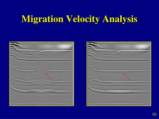
Parameter Extraction Synthetic Data Examples: Migrate a COG; Extract Midpoint Coordinates, Traveltimes, and Incidence Angles.
Distance (km) 0 4 8 12 16 0 1 Depth (km) 2 3 4 Kirchhoff Migration of a COG
Distance (km) 0 4 8 12 16 0 1 Depth (km) 2 3 4 Weighted Kirchhoff Migration of a COG Extra Weight
COG Incidence Angles Distance (km) 0 8 16 0 20 (Degrees) Depth (km) 10 2 4 0
COG Incidence Angles Distance (km) 0 8 16 0 20 (Degrees) Depth (km) 10 2 4 0
COG Traveltimes Distance (km) 0 8 16 3.5 0 (Seconds) Depth (km) 1.75 2 4 0
COG Traveltimes Distance (km) 0 8 16 3.5 0 (Seconds) Depth (km) 1.75 2 4 0
COG S-R Midpoint Coordinates Distance (km) 0 8 16 20 0 Depth (km) (km) 10 2 4 0
COG S-R Midpoint Coordinates Distance (km) 0 8 16 20 0 Depth (km) (km) 10 2 4 0
Distance (km) 0 4 8 12 16 0 1 Depth (km) 2 3 4 Verification of Extracted Parameters
COG S-R Midpoint Coordinates Distance (km) 0 8 16 20 0 Depth (km) (km) 10 2 4 0
COG Traveltimes Distance (km) 0 8 16 3.5 0 (Seconds) Depth (km) 1.75 2 4 0
Verification of Extracted Parameters Trace Midpoint Coordinates 11 13 15 1 Time (sec) Trvaeltimes Extracted 2
Applications • Stationary Phase Migration • Tomographic Velocity Analysis
Stationary Phase Migration SPM uses specular-ray parameters to : • Migrate traces within Fresnel zone • Reject traces out of Fresnel zone • Suppress alias artifacts
Stationary Phase Migration • Algorithm • Synthetic Data Example • Field Data Example
Stationary Phase Migration Operator Schleicher et al. (1997) : Fresnel zone width Minimum Aperture Fresnel Zone Stationary phase point
Stationary Phase Migration • Algorithm • Synthetic Data Example • Field Data Example
Kirchhoff Migration of a COG Distance (km) 0 4 8 12 16 0 1 2 Depth (km) 3 4
Stationary Phase Mig. of a COG Distance (km) 0 4 8 12 16 0 1 2 Depth (km) 3 4
Migration Operator Trace Contributions
Trace Contributions : KM Trace Number 0 150 300 0 Depth (km) 2 4
Trace Contributions : SPM Trace Number 0 150 300 0 Depth (km) 2 4
Trace Contributions : KM Trace Number 0 150 300 0 Depth (km) 2 4
Trace Contributions : SPM Trace Number 0 150 300 0 Depth (km) 2 4
Trace Contributions : KM Trace Number 0 150 300 0 Depth (km) 2 4
Trace Contributions : SPM Trace Number 0 150 300 0 Depth (km) 2 4
Incidence Angle CIG Offset (km) Offset (km) 0 3 0 3 0 70 0 Depth (km) Depth (km) 35 2 2 4 4 0 (Deg)
Incidence Angle CIG Offset (km) Offset (km) 0 3 0 3 0 70 0 Depth (km) Depth (km) 35 2 2 4 4 0 (Deg)
Stacked SPM Image After Muting Distance (km) 0 4 8 12 16 0 1 2 Depth (km) 3 4
Stacked SPM Image Without Muting Distance (km) 0 4 8 12 16 0 1 2 Depth (km) 3 4
Stationary Phase Migration • Algorithm • Synthetic Data Example • Field Data Example
Kirchhoff Migration of a COG Distance (km) 0 2 4 6 8 10 12 14 0 2 Depth (km) 4 6
Stationary Phase Mig. of a COG Distance (km) 0 2 4 6 8 10 12 14 0 2 Depth (km) 4 6
Stacked KM Image Distance (km) 0 2 4 6 8 10 12 14 0 2 Depth (km) 4 6
Stacked SPM Image Distance (km) 0 2 4 6 8 10 12 14 0 2 Depth (km) 4 6
Stationary Phase Mig. vs Wavepath Mig. S G • Both approaches suppress alias artifacts • WM measures emergence angles in the data domain • SPM extracts parameters in the migration domain • SPM extracts more parameters • WM is faster • SPM may be more robust in parameter estimations
Applications • Stationary Phase Migration • Tomographic Velocity Analysis
Steps in Tomographic MVA • Build up Initial Migration Velocity • Migrate Seismic Data • Obtain S & R Coordinates • Find Specular-Ray Paths • Pick Depth Residual Moveouts • Pick Reflector Positions • Update Velocities • Migrate Seismic Data With • Updated Velocities • Repeat Above Steps