Download
1 / 38
690 likes | 1.33k Views
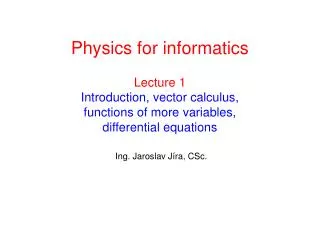
Physics for informatics. Lecture 1 Introduction , vector calculus, functions of more variables, differential equations. Ing. Jaroslav J í ra , CSc. Introduction. Lecturers: prof. Ing. Stanislav Pekárek, CSc., pekarek@fel.cvut.cz , room 49A

E N D
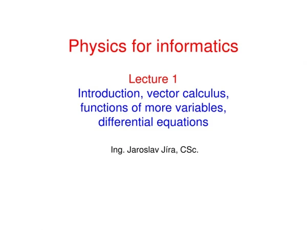
Physics for informatics Lecture 1Introduction, vector calculus, functions of more variables,differential equations Ing. Jaroslav Jíra, CSc.
Introduction Lecturers: prof. Ing. Stanislav Pekárek, CSc., pekarek@fel.cvut.cz , room 49A Ing. Jaroslav Jíra, CSc., jira@fel.cvut.cz , room 42 Source of information:http://aldebaran.feld.cvut.cz/ , section Physics for OI Textbooks:Physics I, Pekárek S., Murla M. Physics I - seminars, Pekárek S., Murla M. Scoring system of the Physics for OI The maximum reachable amount of points from semester is 100. Points from semester go with each student to the exam, where they create a part of the final grade according to the exam rules. Conditions for assessment: - to gain at least 40 points, - to measure specified number of laboratory works, - to submit specified number of partial problems, - to submit semester work
Points can be gained by: - written tests, max. 50 points. Two tests by 25 points max. (8th and 13th week) - semester work for max. 30 points - activity on exercises, partial problems solving, max. 20 points Examination – first part: Every student must solve certain number ofproblems according to his/herpoints from the semester.
Examination - second part: Student answers questions in written form during the written exam. The answers are marked and the total of 30 points can be gained in this way. Then follows oral part of the exam and each student defends a mark according to the table below. The column resulting in better mark is taken into account.
Vector calculus - basics A vector – standard notation for three dimensions Unit vectors i,j,kare vectors of magnitude 1 in directions of the x,y,z axes. Magnitude of a vector Position vector is a vector r from the origin to the current position where x,y,z, are projections of r to the coordinate axes.
Adding and subtracting vectors Multiplying a vector by a scalar Example of multiplying of a vector by a scalar in a plane
Example of addition of three vectors in a plane The vectors are given: Numerical addition gives us Graphical solution:
Example of subtraction of two vectors a plane The vectors are given: Numerical subtraction gives us Graphical solution:
Example of the time derivation of a vector The motion of a particle is described by the vector equation Determine for any time t: a) b) the tangential and the radial accelerations
Time derivation of a vector in the Mathematica -continued What would happen without Assuming and Refine What would happen without Simplify Graphical output of the
Example of the time integration of a vector Evaluate the time dependence of the velocity and the position vector for the projectile motion. Initial velocity v0=(10,20) m/s and g=(0,-9.81) m/s2.
Time integration of a vector in the Mathematica Study of balistic projectile motion, whencomponents of initial velocity are given Projectile motion - trajectory:
Scalar product Scalar product (dot product) – is defined as Where Θ is a smaller angle between vectors a and b and S is a resulting scalar. For three component vectors we can write Geometric interpretation – scalar product is equal to the area of rectangle havinga and b.cosΘas sides.Blue and red arrows represent original vectors a and b. Basic properties of the scalar product
Vector product Vector product (cross product) – is defined as Where Θ is the smaller angle between vectors a and b and n is unit vector perpendicular to the plane containing a and b. Geometric interpretation - the magnitude of the cross product can be interpreted as the positive area Aof the parallelogram having a and b as sides Component notation Basic properties of the vector product
Direction of the resulting vector of the vector productcan be determined eitherby the right hand rule or by the screw rule Vector triple product Geometric interpretation of the scalar triple product isa volume of a paralellepipedV Scalar triple product
Scalar field and gradient Scalar fieldassociates a scalar quantity to every point in a space. This association can be described by a scalar function fand can be also time dependent. (for instance temperature, density or pressure distribution). The gradient of a scalar field is a vector field that points in the direction of the greatest rate of increase of the scalar field, and whose magnitude is that rate of increase. Example: the gradient of the function f(x,y) = −(cos2x + cos2y)2 depicted as a projected vector field on the bottom plane.
Example 2 – finding extremes of the scalar field Find extremes ofthe function: Extremes can be found by assuming: In this case : Answer: there are two extremes
Vector operators Gradient (Nabla operator) Divergence Curl Laplacian
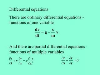
Differential equations The most simple differential equation: where We are looking for the function Solution of such equation is Example: Where x2+C is general solution of the differential equation Sometimes an additional condition is given like that means the function y(x) must pass through a point We have obtained a particular solutiony(x)=x2 -1
First order homogenous linear differential equationwith constant coefficients The general formula for such equation is To solve this equation we assume the solution in the form of exponential function. then If and the equation will change into after dividing by the eλx we obtain aλ+b is the characteristic equation the solution is Where C is a constant resulting from the initial condition
Example of the first order LDE – RC circuit Find the time dependence of the electric current i(t) in the given circuit. Now we take the first derivative of the right equation with respect to time characteristic equation is Constant K can be calculated from initial conditions. We know that general solution is particular solution is
Solution of the RC circuit in the Mathematica Given values are R=1 kΩ; C=100 μF; u=10 V
Second order homogenous linear differential equationwith constant coefficients The general formula for such equation is To solve this equation we assume the solution in the form of exponential function: then If and and the equation will change into after dividing by the eλx we obtain We obtained a quadratic characteristic equation.The roots are
There exist three solutions according to the discriminant D 1) If D>0, the roots λ1,λ2are real and different 2) If D=0, the roots are real and identical λ12 =λ 3) If D<0, the roots are complex conjugate λ1,λ2 where α and ω are real and imaginary parts of the root
If we substitute we obtain This is the solution in some cases, but … Further substitution is sometimes used and then considering formula we finally obtain where amplitude A and phase φ are constants which can be obtained from the initial conditions and ω is angular frequency.This example leads to an oscillatory motion.
Example of the second order LDE – a simple harmonic oscillator Evaluate the displacement x(t) of a body of mass m on a horizontal spring with spring constant k. There are no passive resistances. If the body is displaced from its equilibrium position (x=0), it experiences a restoring force F, proportional to the displacement x: From the second Newtons law of motion we know Characteristic equation is We have two complex conjugate roots with no real part
The general solution for our symbols is No real part of λmeans α=0, and omega in our case The final general solution of this example is Answer: the body performs simple harmonic motion with amplitude A and phase φ. We need two initial conditions for determination of these constants. These conditions can be for example From the first condition From the second condition The particular solution is
Example 2 of the second order LDE – a damped harmonic oscillator The basic theory is the same like in case of the simple harmonic oscillator, but this time we take into account also damping. The damping is represented by the frictional force Ff, which is proportional to the velocity v. The total force acting on the body is The following substitutions are commonly used Characteristic equation is
Solution of the characteristic equation where δ is damping constant and ωis angular frequency There are three basic solutions according to the δ and ω. 1) δ>ω.Overdamped oscillator. The roots are real and different 2) δ=ω.Critical damping. The roots are real and identical. 3) δ<ω.Underdamped oscillator. The roots are complex conjugate.
Damped harmonic oscillator in the Mathematica Damping constant δ=1[s-1], angular frequencyω=10 [s-1]
Damped harmonic oscillator in the Mathematica All three basic solutions together for ω=10 s-1Overdamped oscillator, δ=20 s-1Critically damped oscillator, δ=10 s-1Underdamped oscillator, δ=1 s-1