Download
1 / 14
160 likes | 255 Views
Learn about differential equations in physics, including first and second-order homogenous linear equations with constant coefficients. Explore examples of solving differential equations in RC circuits and harmonic oscillators. Understand the theory behind damped harmonic oscillators. Discover how to find solutions using characteristic equations and initial conditions.

E N D
Physics for informatics Lecture 2Differential equations Ing. Jaroslav Jíra, CSc.
Differential equations The most simple differential equation: where We are looking for the function Solution of such equation is Example: Where x2+C is general solution of the differential equation Sometimes an additional condition is given like that means the function y(x) must pass through a point We have obtained a particular solutiony(x)=x2 -1
First order homogenous linear differential equationwith constant coefficients The general formula for such equation is To solve this equation we assume the solution in the form of exponential function. then If and the equation will change into after dividing by the eλx we obtain aλ+b is the characteristic equation the solution is Where C is a constant resulting from the initial condition
Example of the first order LDE – RC circuit Find the time dependence of the electric current i(t) in the given circuit. Now we take the first derivative of the right equation with respect to time characteristic equation is Constant K can be calculated from initial conditions. We know that general solution is particular solution is
Solution of the RC circuit in the Mathematica Given values are R=1 kΩ; C=100 μF; u=10 V
Second order homogenous linear differential equationwith constant coefficients The general formula for such equation is To solve this equation we assume the solution in the form of exponential function: then If and and the equation will change into after dividing by the eλx we obtain We obtained a quadratic characteristic equation.The roots are
There exist three solutions according to the discriminant D 1) If D>0, the roots λ1,λ2are real and different 2) If D=0, the roots are real and identical λ12 =λ 3) If D<0, the roots are complex conjugate λ1,λ2 where α and ω are real and imaginary parts of the root
If we substitute we obtain This is the solution in some cases, but … Further substitution is sometimes used and then considering formula we finally obtain where amplitude A and phase φ are constants which can be obtained from the initial conditions and ω is angular frequency.This example leads to an oscillatory motion.
Example of the second order LDE – a simple harmonic oscillator Evaluate the displacement x(t) of a body of mass m on a horizontal spring with spring constant k. There are no passive resistances. If the body is displaced from its equilibrium position (x=0), it experiences a restoring force F, proportional to the displacement x: From the second Newtons law of motion we know Characteristic equation is We have two complex conjugate roots with no real part
The general solution for our symbols is No real part of λmeans α=0, and omega in our case The final general solution of this example is Answer: the body performs simple harmonic motion with amplitude A and phase φ. We need two initial conditions for determination of these constants. These conditions can be for example From the first condition From the second condition The particular solution is
Example 2 of the second order LDE – a damped harmonic oscillator The basic theory is the same like in case of the simple harmonic oscillator, but this time we take into account also damping. The damping is represented by the frictional force Ff, which is proportional to the velocity v. The total force acting on the body is The following substitutions are commonly used Characteristic equation is
Solution of the characteristic equation where δ is damping constant and ωis angular frequency There are three basic solutions according to the δ and ω. 1) δ>ω.Overdamped oscillator. The roots are real and different 2) δ=ω.Critical damping. The roots are real and identical. 3) δ<ω.Underdamped oscillator. The roots are complex conjugate.
Damped harmonic oscillator in the Mathematica Damping constant δ=1[s-1], angular frequencyω=10 [s-1]
Damped harmonic oscillator in the Mathematica All three basic solutions together for ω=10 s-1Overdamped oscillator, δ=20 s-1Critically damped oscillator, δ=10 s-1Underdamped oscillator, δ=1 s-1