Download
1 / 54
550 likes | 768 Views
A Drop of the Hard Stuff: How Maxwell Created His Equations, What They Mean, and How They Predicted the Discovery of Radio. Peter Excell Professor of Communications. Outline. Mathematical Physics delivering real benefits Using computers to make it ‘easier’ Implications. “Pre-requisites”.

E N D
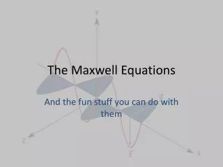
A Drop of the Hard Stuff: How Maxwell Created His Equations, What They Mean, and How They Predicted the Discovery of Radio Peter Excell Professor of Communications
Outline • Mathematical Physics delivering real benefits • Using computers to make it ‘easier’ • Implications
“Pre-requisites” • Differentiation • Electric & Magnetic fields • Electric circuits
“Maxwell’s Equations” So: ? No!
Electromagnetic Waves • Theories of electric and magnetic fields evolved independently of the main theories of optics, but JAMES CLERK MAXWELL showed how they were related. • This was one of the greatest achievements of Physics, particularly as it started as an abstruse mathematical theory but went on to become a major applied technology which has had a major effect in shaping the modern world: Radio Waves
Electromagnetic Waves This is equivalent to today’s modern physics when/if it produces results which are taken forward to everyday practical applications, e.g.: • Superstring Theory • The Large Hadron Collider • Stephen Hawking’s stuff
Electromagnetic Fields • Oersted and Ampere showed how an electric current could create a magnetic field, causing ‘action at a distance’. • Faraday showed how a magnetic field could create a current, but only if it was varying in time. • Maxwell generalised Faraday’s and Ampere’s Laws, combined them, and discovered an equation for travelling electromagnetic waves.
An approximate explanation of how Maxwell discovered the Electromagnetic Wave Equation(Developed for first-year Elec. Eng. Students in the 1990s…)
Maxwell’s generalisation of Faraday’s Law of electromagnetic induction Induced voltage: is the total magnetic flux, in Webers (Wb), at right-angles to the wire loop. But = BA, where B is magnetic flux density (Wb/m2 or T) and A is coil area.
Generalising Faraday Let A = xy, then: Now suppose the ‘voltmeter’ side is opened up so that we just see an electric field, E, across a gap. The electric field in the gap is approximately given by:
Generalising Faraday Differentiate both sides with respect to x: this has to be a partial derivative because E and B are functions of both time and position: This is a simple statement of Maxwell’s generalisation of Faraday’s Law.
Generalising Faraday The complete form is: Park that. ………………….. Now we look at Ampère’s Law:
Generalising Ampère Ampère’s Law describes the magnetic flux set up by a current-carrying wire: The current I sets up a magnetic flux density B:
Generalising Ampère Why? 1. Because Ampère found that current-carrying circuits exerted a force on each other, due to their magnetic fields, inversely proportional to distance and proportional to the current.
Generalising Ampère • Why? • 2. Because B = H by definition: • B is magnetic flux density • H is magnetic field strength • is permeability (a constant of ‘space’, linking the force produced by magnetic fields to the current creating them)
Generalising Ampère Now suppose that there is a capacitor in the circuit: There is no current in the gap in the capacitor (the dielectric), but experiment (and reasoning) shows there must still be a magnetic flux and field.
Generalising Ampère What is the equivalent of ordinary conduction current in the capacitor gap? Start with the basic equation for a capacitor: For a parallel-plate capacitor (ignoring ‘fringing’): Where g is the gap width
Generalising Ampère is permittivity (another constant of ‘space’, linking the force produced by electric fields to the voltage creating them)
Generalising Ampère Now combine: This is the so-called ‘Displacement Current’ – a key Maxwell innovation.
Generalising Ampère The equivalent current density, J, (A/m2) is: because D (electric flux density) = E
Generalising Ampère Now go back to the circuitand take a magnified view of part of the wire: Now consider the wire to be a thin-walled tube so that all current is forced to flow on its surface:
Generalising Ampère Take ‘r’ to be equal to the ‘wire’ radius, so we are observing the magnetic fields right on the metal surface: hence: H = Jx Differentiating with respect to x:
Generalising Ampère Now suppose there is a gap in the tube, forming a narrow capacitor: In the gap, J is replaced by dD/dt, but this should now be written as a partial derivative, to allow for spatial variations.
Generalising Ampère In a general case, both conduction and displacement currents may be present, hence: This is a simplified form of the Maxwell-Ampère Equation, Maxwell’s generalisation of Ampère’s Law.
Generalising Ampère The full vector version is:
The Wave Equation In vacuum (or air) there can be no conduction current and the Maxwell-Ampère equation reduces to: But Faraday’s Law (as generalised by Maxwell) gave us another such equation: Notice the symmetry…
The Wave Equation Differentiate the Faraday-Maxwell equation with respect to x: F-M: Diff: The exchange in the order of the differentiations is allowable if there is no mechanical movement. Now we can combine this equation with the Maxwell-Ampère equation above to give an equation in E as the only field component.
The Wave Equation DifferentiatedF-M: M-A: Eliminate H: Note: the electric fields in the two equations are not quite the same, and we have to change the sign of one when combining them, by dropping the minus sign. This fudge doesn’t arise when the full vector treatment is used: a weakness of the very simplified treatment used here.
The Wave Equation This is a WAVE EQUATION for electric fields: a momentous result. This is a double simple harmonic motion type of equation with respect to x and t simultaneously. It is satisfied by solutions which oscillate sinusoidally with respect to x and t simultaneously, e.g.
The Wave Equation The term has the dimensions of time, i.e. distance/speed, so is a speed. • ( is a frequency) • and can be found from laboratory experiments with electromagnets and capacitors: • = 4 x 10⁻⁷ H/m, and = 8.85 x 10⁻¹² F/m, so: = 2.998x10⁸ m/s THE SPEED OF LIGHT!
The Wave Equation This truly remarkable result, first derived by Maxwell, showed that electromagnetic waves could exist, which travelled at the speed of light. It strongly implied that light was such an electromagnetic wave (later proved to be so), - but that light-like waves could exist over a much wider spectrum than was then known (infrared-ultraviolet).
The Wave Equation • It also implied that such waves could exist at low frequencies, in which case they: • Could bend round corners and over the horizon • B. Could go through clouds and fog (and walls) • C. Could be created by ordinary electric circuits
Exploitation James Clerk Maxwell died in 1879, before he could test his theory. The existence of such ‘radio’ waves was first demonstrated by Heinrich Hertz, working in Germany, in 1888. Hertz’ experiments were only on a laboratory scale, and he also died young. Radio was commercialised by Guglielmo Marconi who first transmitted information in a radio signal in 1895 and got a signal across the Atlantic in 1901.
Exploitation Marconi found influential backers…. The invention of the radio valve helped the technology: the imperative of working with very weak signals initiated electronics. The sinking of the Titanic showed the importance of radio in ships. The First World War gave a massive boost to radio. After the war, entertainment applications drove the technology. TV – Radar – Satellites – Mobile phones…
Einstein The wave has a velocity, but with respect to what? It was thought that space was filled with aether, which carried light waves, even in a vacuum. This would mean that tests of the speed of light would give different results as the Earth moved through space: this was found not to be the case (Michelson-Morley Experiment).
Einstein Lorentz proposed that everything, including the measuring equipment, ‘shrank’ in the direction of movement through the aether, so that speed change would be undetectable (‘Lorentz Contraction‘). Albert Einstein showed that the aether was not necessary…
Einstein Albert Einstein showed that the aether was not necessary if it was accepted that the speed of light was a fundamental constant of the universe. Since the speed is based on the constants and this seems reasonable. But since velocity = distance/time it means that distance and time are no longer absolute quantities.
Einstein This leads to the very surprising effect of Time Dilation which means that clocks appear to run slower in systems moving relative to the observer. This is the basis of Einstein’s Special Theory of Relativity: a severe upset to ‘common sense’ understanding!
Einstein Note that the theory really grew from consideration of Maxwell’s work on the electromagnetic nature of light. The well-known equation E = mc2 is a secondary consequence.
Using computers to make it ‘easier’ Differentiation can be replaced by a ‘finite-difference approximation’, e.g.: These ‘discretised’ versions can easily be programmed into a computer, but space and time have to be chopped up into tiny segments, so the sums are easy(ish), but there can be billions of them…
Using computers to make it ‘easier’ • Another approach: • Convert Maxwell’s Equations to integral forms using Stokes’ and Gauss’ theorems, then form an ‘Integral Equation’ approach. • Equivalent to the ‘action at a distance’ view of field phenomena. • The finite difference approach is equivalent to Faraday’s view of a pervasive field. • This gets down to the epistemology of science…
Finite-difference model of a row of biological cells with a 900MHz wave incident from the left
Integral-equation model of detailed current distribution on self-resonant coils
Finite-difference model of a sphere simulating a human head, with a 900MHz wave incident from the left.
Finite-difference model of a human head, with mobile phone adjacent at bottom
Finite-difference grid structure for a human head, with mobile phone and human hand models
Structure for a hybrid model, using finite-difference for the sphere (simulating a head) and integral-equation method for the phone and antenna