Download
1 / 33
340 likes | 412 Views
Explore the fundamental concepts of ray theory and scattering theory in seismic wave analysis, including derivation of ray equations, Eikonal equation, and the Projection Slice Theorem. Learn about the Green's function, scattering potential, and wave equation applications in waveform tomography.

E N D
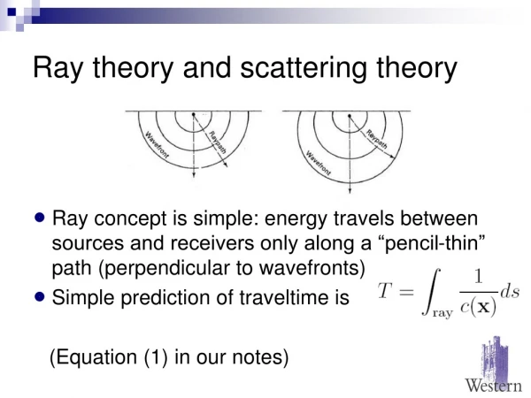
Ray theory and scattering theory • Ray concept is simple: energy travels between sources and receivers only along a “pencil-thin” path (perpendicular to wavefronts) • Simple prediction of traveltime is (Equation (1) in our notes)
Ray theory and scattering theory • This picture is a fiction: Seismic energy is scattered in all directions, in a complicated way • Ray picture is a very simplified (and very useful) model • The model derives directly from the wave equation …
Derivation of ray equation • The ray integral can be obtained directly from the acoustic wave equation: • or, in the frequency domain
Derivation of ray equation • assume the shape of the pulse does not change • an impulse (delta) changes in amplitude and time • constant time surfaces (wavefronts) are • rays are normal to these surfaces • transforming into the frequency domain • this implies no dispersion (no frequency dependence)
Derivation of ray equation • We now substitute into the wave equation • This yields (after division by ω2) • No approximations made so far …
Derivation of ray equation • We now make a key approximation in: • We assume that ω approaches infinity (this is the fundamental reason for the limitation of ray methods) • This assumption allows us to retain only zeroth order terms, leaving: (the “Eikonal” equation)
Derivation of ray equation The “Eikonal” equation implies that is a unit vector. • This vector must be normal to wavefronts (constant time surfaces) • Thus by definition is parallel to rays
Derivation of ray equation The unit vector can be written as (where dr is a a tangent along the ray, with length ds). Thus Take dot product with : The LHS is and the RHS is simply
Derivation of ray equation The unit vector can be written as (where dr is a a tangent along the ray, with length ds). Thus or Since τdefines the constant traveltime surfaces (the wavefronts), integration of this equation along the ray gives us (Equation (1) in our notes, again)
has the same form as Projection slice theorem • f ^ is the “projection data”, f is the “model”, and the straight line L is defined by • this is a “Radon transform”
p k Projection slice theorem • find the inverse Radon transform using Fourier transforms (of the model, and of the data) • 1D Fourier transform of the data:
Projection slice theorem • 2D Fourier transform of the model:
Projection slice theorem • This can be written: • we now take the 1D Fourier transform of both sides (i.e., of the data) …
Projection slice theorem • the 1D Fourier transform of both sides (i.e., of the data): the “Projection Slice Theorem”
Projection slice theorem • this is an inverse Radon transform (in the Fourier domain) • to find the model, fill-in the model Fourier space along a series of lines • with enough projections, we eventually know the model • finally, carry out an inverse Fourier transform • concept is fundamental in tomography • there are problems with this approach in practice, so other methods are more common
Projection slice theorem Recall our two major assumptions • high frequency, “asymptotic ray” assumption – Geometrical optics • assumption of straight rays (homogeneous background medium) • curved ray traveltime tomography is the standard approach • we now investigate how we may relax the asymptotic ray assumption
Scattering of seismic waves • Return to the acoustic wave equation: • add a point source term (the response to the point source is the “Green’s function”)
Scattering of seismic waves • the Green’s function for a single frequency is the response to a point source vibrating at that frequency
Scattering of seismic waves • For problems with an extended source: -
Scattering of seismic waves • What is the change if we perturb the velocity? • “split” the model into two parts: • o(x) is the “object” function, or “scattering potential” • introduce Go as the solution to:
Scattering of seismic waves • We now “split” the wavefield into two parts: • substituting these into the wave equation yields:
- Scattering of seismic waves • the new wave equation describes the scattered field – the scattering potential “creates” the field as if there were a distribution of sources • there is also an integral form for this equation:
- Scattering of seismic waves - • the integral form is non-linear (total field appears on the RHS) • standard approximation is to replace the total field on the RHS, with the background (“incident”) field G0 • this is the first Born approximation, valid for weak scattering • no restriction on background velocity, provided we can calculate the background field
Waveform tomography 150 m Frequency 300 Hz Wavelength = 10 m 300 m s2(r) ω
Waveform tomography 150 m Frequency 300 Hz Wavelength = 10 m 300 m s2(r) ω
Fresnel zone width L 38 m (300 Hz) Waveform tomography 150 m Frequency 300 Hz Wavelength = 10 m “Seismic wavepath” (Woodward and Rocca, 1989, 1992) 300 m s2(r) ω
ko=ω/co Generalized projection slice theorem - • as before, we want to invert the relationship and find the target (in this case, the scattering potential) • with the Radon transform we assumed straight rays • here we assume homogeneous background • far from the sources/receivers, G0 are plane waves • s and r are unit vectors from the source and receiver locations
with yields - Generalized projection slice theorem - • i.e., we multiply the target by a sinusoid, and integrate • this is Fourier transformation (extraction of a particular wavenumber of the target)
kz - k s k (r - s) k r kx k s Born scattering in (kx,kz) (e.g., Wu and Toksoz, 1987) Born scattering in the frequency domain x z
- Generalized projection slice theorem - • the integral is a Fourier transformation, so • O(kx,kz) is the 2D Fourier transform of the object • thus the single frequency, single plane wave response yields one Fourier component of the target • by using additional plane wave experiments we eventually can know the Fourier transform of the model • finally, carry out an inverse 2D Fourier transformation
Generalized projection slice theorem - • This result is the “Generalized Projection Slice” theorem • the waves are scattered in a range of directions, sweeping out “Ewald” circles
- Projection slice theorems