Download
1 / 45
450 likes | 676 Views
Analysis of Gene Networks and Signaling Pathways Based on Gene Expression and Proteome Data. Marek Kimmel Rice University Houston, TX, USA kimmel@rice.edu. Outline. Basics: gene expression vs. protein abundance. Perceptron analysis of gene networks

E N D
Analysis of Gene Networks and Signaling Pathways Based on Gene Expression and Proteome Data Marek Kimmel Rice University Houston, TX, USA kimmel@rice.edu
Outline • Basics: gene expression vs. protein abundance. • Perceptron analysis of gene networks • Proteomic analysis of FGF-2 signaling in breast cancer
Now that we have the sequence of the HumanGenome – What Next?
Bioinformatics Basic Sciences Clinical Sciences Proteomics Genomics Structural Biology Molecular Medicine
30,000 Genes make up only 3% of the genome BCM- HGSC
Measuring Gene Expression: Oligonucleotide Gene Microarrays Affymetrix GeneChips™ • A Probe Pair consists of a Perfect Match (PM) & a Mismatch (MM). • There are typically 20 Probe Pairs in a Probe Set. • A Probe Set usually corresponds to a single gene. • The Affymetrix 95A human GeneChip contains 12,626 Probe Sets. • Thus, there are almost 500,000 Probe Cells on a GeneChip.
Oligonucleotide Gene Microarrays Affymetrix GeneChips™ Each probe is 25 nucleotides long
5’ GAATTCAGTAACCCAGGCATTATTTTATCCTCAAGTCTTAGGTTGGTTGGAGAAAGATAACAAAAAGAAACATGA TTGTGCAGAAACAGACAAACCTTTTTGGAAAGCATTTGAAAATGGCATTCCCCCTCCACAGTGTGTTCACAGTGT GGGCAAATTCACTGCTCTGTCGTACTTTCTGAAAATGAAGAACTGTTACACCAAGGTGAATTATTTATAAATTAT GTACTTGCCCAGAAGCGAACAGACTTTTACTATCATAAGAACCCTTCCTTGGTGTGCTCTTTATCTACAGAATCC AAGACCTTTCAAGAAAGGTCTTGGATTCTTTTCTTCAGGACACTAGGACATAAAGCCACCTTTTTATGATTTGTT GAAATTTCTCACTCCATCCCTTTTGCTGATGATCATGGGTCCTCAGAGGTCAGACTTGGTGTCCTTGGATAAAGA GCATGAAGCAACAGTGGCTGAACCAGAGTTGGAACCCAGATGCTCTTTCCACTAAGCATACAACTTTCCATTAGA TAACACCTCCCTCCCACCCCAACCAAGCAGCTCCAGTGCACCACTTTCTGGAGCATAAACATACCTTAACTTTAC AACTTGAGTGGCCTTGAATACTGTTCCTATCTGGAATGTGCTGTTCTCTT 3’ Chop into short pieces suitable for hybridizing to 25mers on GeneChip 5’ GAATTCAGTAACCCAGGCATTATTT|TATCCTCAAGTCTTAGGTTGGTTGG|AGAAAGATAACAAAAAGAAACATGA| TTGTGCAGAAACAGACAAACCTTTT|TGGAAAGCATTTGAAAATGGCATTC|CCCCTCCACAGTGTGTTCACAGTGT| GGGCAAATTCACTGCTCTGTCGTAC|TTTCTGAAAATGAAGAACTGTTACA|CCAAGGTGAATTATTTATAAATTAT| GTACTTGCCCAGAAGCGAACAGACT|TTTACTATCATAAGAACCCTTCCTT|GGTGTGCTCTTTATCTACAGAATCC| AAGACCTTTCAAGAAAGGTCTTGGA|TTCTTTTCTTCAGGACACTAGGACA|TAAAGCCACCTTTTTATGATTTGTT| GAAATTTCTCACTCCATCCCTTTTG|CTGATGATCATGGGTCCTCAGAGGT|CAGACTTGGTGTCCTTGGATAAAGA| GCATGAAGCAACAGTGGCTGAACCA|GAGTTGGAACCCAGATGCTCTTTCC|ACTAAGCATACAACTTTCCATTAGA| TAACACCTCCCTCCCACCCCAACCA|AGCAGCTCCAGTGCACCACTTTCTG|GAGCATAAACATACCTTAACTTTAC|AACTTGAGTGGCCTTGAATACTGTT|CCTATCTGGAATGTGCTGTTCTCTT 3’ mRNA Preparation DNA Sequence for IL-8 Attach chromophore, then inject onto the GeneChip
AGTCGGATTAAGCGCTATACGGTTC | AGTCGGATTAAGTGCTATACGGTTC | AGTCGGATTAAGCGCTATACGGTTC | AGTCGGATTAAGGGCTATACGGTTC | AGTCGGATTAAGCGCTATACGGTTC | AGTCGGATTAAGGGCTATACGGTTC | AGTCGGATTAAGCGCTATACGGTTC | AGTCGGATTAAGGGCTATACGGTTC | AGTCGGATTAAGTGCTATACGGTTC | AGTCGGATTAAGCGCTATACGGTTC | AGTCGGATTAAGAGCTATACGGTTC | AGTCGGATTAAGCGCTATACGGTTC | AGTCGGATTAAGCGCTATACGGTTC | AGTCGGATTAAGAGCTATACGGTTC | AGTCGGATTAAGAGCTATACGGTTC | AGTCGGATTAAGCGCTATACGGTTC | |TCAGCCTAATTCGCGATATGCCAAG |TCAGCCTAATTCGCGATATGCCAAG PM MM Affymetrix Hybridization X
AGTCGGATTAAGTGCTATACGGTTC | AGTCGGATTAAGCGCTATACGGTTC | AGTCGGATTAAGGGCTATACGGTTC | AGTCGGATTAAGCGCTATACGGTTC | AGTCGGATTAAGCGCTATACGGTTC | AGTCGGATTAAGGGCTATACGGTTC | AGTCGGATTAAGCGCTATACGGTTC | AGTCGGATTAAGGGCTATACGGTTC | AGTCGGATTAAGTGCTATACGGTTC | AGTCGGATTAAGCGCTATACGGTTC | AGTCGGATTAAGCGCTATACGGTTC | AGTCGGATTAAGAGCTATACGGTTC | AGTCGGATTAAGAGCTATACGGTTC | AGTCGGATTAAGCGCTATACGGTTC | AGTCGGATTAAGAGCTATACGGTTC | AGTCGGATTAAGCGCTATACGGTTC | |TCAGCCTAATTCGCGATATGCCAAG |TCAGCCTAATTCGCGATATGCCAAG PM MM Affymetrix Hybridization Forms duplex with complementary strand X Match Mismatch!
1,662 Probe Cell Intensities Average Difference = S(PM – MM)/Pairs in Average
http://rana.lbl.gov/ http://www.bioinfo.utmb.edu/ http://www.microarrays.org/software.html Measuring Gene Expression“Spotted DNA Microarrays” • Each spot is the cDNA for a specific gene. • RNA from the experimental sample is labeled with Cy5 red fluorescent dye. • RNA from the reference sample is labeled with Cy3 green fluorescent dye. • Fluorescent intensity ratios (Cy5/Cy3) are measured.
Disease, Pathogens, Drugs, etc… Where Do We Get the Data? Microarray analyzed for spot intensities Gene co-expression patterns mRNA expressed in response to stimulus mRNA collected and hybridized onto microarray cDNA Gene Microarray
Method • Get mRNA samples from multiple conditions. • Hybridize to DNA microarrays. • Measure intensities. • Cluster. • Analyze results. • Design new experiment.
Discrimination between samples • Green is “down”. • Red is “up”. • We can differentiate clearly between tumor and normal tissue. • Can we find differences between progressing and non-progressing tumors?
Problematic quality of data • Note the large dynamic range. • And the verylarge number of data points. • And the limited information content.
Proteomics • Is to protein expression what genomics is to gene expression. • Due to variations like post-translational modifications, there are many more proteins than genes.
Proteomics • Holds new promise for the future understanding of complex biological systems. • Post-translational modifications include: • Phosphorylation • Glycosylation • Oxidation • Many challenges remain, e.g. isolating, identifying, characterizing, and quantifying small amounts of a very large number of varieties of proteins • Currently, we primarily use 2D gels and mass spectroscopy.
Protein Separation Using 2D Gel Electrophoresis • Protein analysis uses a diseased or treated sample and a control sample. 2D gel electrophoresis is performed for each sample to separate proteins based on their molecular weight and charge. • Black marks on the gel images indicate a protein or cluster of proteins and are referred to as "features." • The x-axis is the Isoelectric point (pI) which is analagous to pH, while the y-axis is molecular weight (Mw) or size. http://www.incyte.com/proteomics/tour/separation.shtml
Protein Analysis • Gels are fixed and stained with a fluorescent dye, then scanned. • Expression levels are measured based on the size of each feature on the gel. • Provides information about those proteins which are up and down-regulated, including how their abundance changed. http://www.incyte.com/proteomics/tour/analysis.shtml
Protein Analysis http://www.incyte.com/proteomics/tour/analysis.shtml
Protein Characterization • Proteins are excised from the gel and treated with a succession of enzymes that cut amino acid chains into short polypeptides about 5-10 amino acids in length. • The polypeptide fragments for each protein are then separated by capillary electrophoresis and analyzed using rapid-throughput mass spectrometry. • At this point, we know the amino acid sequence of the polypeptide fragments, their mass, as well as post-translational modifications that occurred such as glycosylation and phosphorylation.
Systems Biology • Consolidates genomics and proteomics differential expression data into a systematic description of pathways. • Signaling pathways. • Inflammatory response pathways. • Metabolic pathways. • Etc… • Potential for understanding the interrelationships between genes, proteins, and disease and identifying potential therapeutic targets.
Gene Expressionvs. Protein Abundance • What exactly are we measuring? • What is the relationship between • “level of gene expression” and • “abundance of proteins” ?
Balance equations In the steady state, for a given genei
Complicating Factors • For any gene, product (protein) abundance is not necessarily proportional to the relative expression level, even under “steady state” . • Products do not follow 1-order elimination kinetics. Instead they enter into complicated interactions with each other and with external factors.
Application:Identification of Gene Networks General ideas: • Level of expression of a gene affects levels of expressions of other genes • Only three levels possible: • Normal (0) • Over-expression (1) • Under-expression (-1) • Data: Arrays of perturbed expression levels in a set of genes • Model: Perceptron (simplest neural net)
Reference Kim et al. (2000) “General nonlinear framework for the analysis of gene interaction via multivariate expression arrays” Journal of Biomedical Optics 5, 411–424
Data table • Perceptron function: • g(.) is sigmoidal, • X’s and Y quantized to 3 levels
Training: Estimating coefficients a so that a coefficient of determination () is maximized. • Of all possible dependencies, only these with above threshold, are retained.
ApplicationFGF-2 Signaling Pathways and Breast Cancer General ideas: • Use 2-D protein gels and mass spectrometry to measure abundance changes of proteins in cancer cells, relative to normal cells. • Use perturbed systems to draw conclusions on some specific signaling pathways. • Example: Signaling pathways of one of the Fibroblast growth factors (FGF-2) in breast cancer.
Reference Hondermarck et al. (2001) “Proteomics of breast cancer for marker discovery and signal pathway profiling” Proteomics 1 , 1216–1232
Figure 2. Silver stained 2-DE profile of MCF-7 breast cancer cells. The major proteins were determined by MALDI-TOF and MS/MS after trypsin digestion.
Figure 3 MALDI-TOF and MS/MS spectra obtained for HSP70. (A) MALDI-TOF and (B) MS/MS analysis of peak m/z 1488.5 was performed. The letters labeling the peaks are the single letter code for the amino acids identified by MS/MS. Database searching allowed the identification of HSP70.
Figure 5 2-D patterns showing the down-regulation of 14-3-3 sigma (indicated by an arrow) in seven representative breast tumor samples (C–I)
Design of experiments • Previously depicted: “abundance proteomics”, no clues as to how things work. • “Functional proteomics” • Use perturbations of the hypothetical causal factor. • Measure not simply abundance but characteristics indicating, e.g., • Synthesis rates • Activation
Figure 7 Changes of protein synthesis induced by FGF-2 stimulation in MCF-7 breast cancer cells. 35 S-labeled proteins from unstimulated (A, C) or stimulated (B, D) MCF-7 cells were separated by 2-DE and 2-D gels were subjected to autoradiography.
Credits • Bruce Luxon (UTMB, Galveston, TX) • George Weinstock (BCM, Houston, TX) • Guy de Maupassant [“three major virtues of a French writer: clarity, clarity, and clarity”]