Effect of Flow-Induced Exchange in Hyporheic Zones on Longitudinal Transport of Solutes

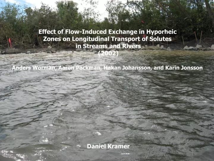
1. Effect of Flow-Induced Exchange in Hyporheic Zones on Longitudinal Transport of Solutes in Streams and Rivers (2002) Anders Worman, Aaron Packman, Hakan Johansson, and Karin Jonsson Daniel Kramer

2. (2) IntroductionTerms For Discussion • Solute (uptake, residence time, longitudinal transport, and spatial variation) • Moment Methods • Solute Break-through Curves • PDF – Probability Density Function • Log Normal Probability • Closed Form Solutions

3. (3) Purpose of Study • Evaluation of Hyporheic Exchange Using Solutes • To Better Understand Transport and Storage of Solutes in Stream • Compare to a theoretical solute model (i.e. Transient Storage Model) • Coupled with a physically based flow-induced uptake model (i.e. Pumping Exchange) • Compare against real measurement data as obtained for a 30 km reach of stream (Sava Brook) in Uppland County, Sweden

4. (4) Evaluation Steps • Review Previous Model Approaches (Diffusive and First Order Exchange) • Couple these solute mass flux assumptions with a Hyporheic exchange flux assumption • This combination allows for a solute break-through curve to be developed. • This can then give various residence times depending on mathematical approach for comparison “couple a physically based representation of flow-induced uptake in the Hyporheic zone with a model for the longitudinal in-stream solute transport.”

5. (5) TheoryExchange Models • First order mass transfer relationships • Parameterization of all mechanisms governing mixing. VS. • Diffusive process • Does not have a hydro mechanical mechanism – entirely non-mechancial

6. (6) TheoryTransport of Solutes • Controlled by: • Exchange with neighboring Hyporheic zone/wetlands • Sorption on to particle matter • Biogeochemical reactions • Must understand these interactions for overall understanding of the transport and fate of nutrient, chemicals, contaminants, etc.

7. (7) Theory -Transient Storage Model (TSM) • Theory of Transport in Streams with Hyporheic Exchange include • Formulated as first order mass transfer and is defined by: • Exchange coefficient • Storage zone depth • Yields - Residence Time of Solute • Flow Direction (GW versus River) • Slope Gradient • Diffusion Problems include unrealistic/over-simplified: cannot account for natural variability and must use multiple exchange rates.

8. (8) TheoryBenefit of Models • Provide a simplified model with a mathematical framework.

9. (9) TheoryProblems with Models • Diffusion Model - Includes the order of magnitude differences between effective diffusive coefficients and molecular diffusion coefficients. • Both models are crude representations – oversimplified. • Require reach specific data to be obtained – costly and timely

10. (10) Hyporheic Exchange – Advection Pumping

11. (11) Hyporheic Exchange – Solute Mass Flux & Hyporheic Exchange Flux Equation 1 = Solute Mass Flux Equation 2 = Hyporheic Exchange Flux Equation 1 + Equation 2 = allow for solute breakthrough curves to be Calc’d per input data of in-stream transport parameters and residence times THIS IS THE ADVECTION STORAGE PATH MODEL or ASP Model

12. (12) Residence Time PDFs • Pumping Exchange Models – Advection Storage Path Model (ASP) • Approximate of flat surface and sinusoidal pressure variation. Mean Depth Hyporheic Zone and Wavelength

13. (13) Residence Time PDF Advection Pump Model ALL Are Close to the Same General Time Log Normal Exponential Simulated TSM Model Pump Model

14. (14) Residence Time PDF Different Models Can Be used to predict Different Transports Single Flow Path Model

15. (15) Closed Form Solutions • Derivation revealed that T and F are controlling Factors (Eq 7 through 10)

16. (16) Closed Form Solutions

17. (17) Closed Form Solutions Temporal Moments can be expressed as co-efficients to T(Eq 12 through 15)

18. (18) SAVA BROOK EXPERIMENT • Tritium as main tracer • Injected for 5.3 hours (how not really discussed?) • Measured at 8 stations along 30 km stretch (no spatial indication?) • Discharge increased along stretch by factor of 4.85 • Water depth and discharge – fairly constant • Took hydraulic conductivity measurements along river to provide plus minus 20% accuracy at a 95% confidence interval

19. (19) SAVA BROOK EXPERIMENT • 85 cross sections geometries defined • Slug test at 3 and 7 cm along 4 to 5 verticals lines/locations • Performed weighted average on these tests to get permeability

20. (20) SAVA BROOK EXPERIMENT

21. (21) SAVA BROOK EXPERIMENT

22. (22) Sava Brook Experiment

23. (23) SAVA BROOK EXPERIMENT Once water enters it is retained in the hyporheic zone for a relatively long time

24. (24) Model Versus Data Points

25. (25) Model Versus Data Points

26. (26) Equating to state variables Review of land type per state variables of a stream showed land use may control Hyporheic exchange - (through differences in channel morphology etc.)

27. (27) Conclusions • The ASP model which is transient combined with advection pumping predicted correctly when compared to Sava Brook • Transient systems best generally analyzed by exponential PDF’s • Advection flows tend to dominates Sava Brook and match well with Log-normal PDF’s so best for streams with pump exchange • Based on Froude number you could potentially analyze other streams - exchange rate increase and residence time decrease with decreasing Froude number.

28. (28) Variables • I am not sure if they ran monte-carlo simulations or just solved for the equations to find probability factors? • Log normal vs exponential – Why, is it because K is generally on a log scale and that is a major factor. Or because co-efficients of diffusion are exponential?

29. (29) Questions & Missing Data? • Missing area description • No real talk of geology, or location images and figures • Specific maps of reach also missing, no spatial image of where measurements were taken • Looking at graphs they need some legend work so I can identify what is what