Download
1 / 39
390 likes | 494 Views
Lesson Four: Student t Distribution and Comparing Samples. Hypotheses. Do You Remember the Coefficient of Variation? We looked at the three samples of BRUS, comparing to the total. We wondered if they were significantly different from each other. Books R US Sample Coefficient of Variation.

E N D
Hypotheses Do You Remember the Coefficient of Variation? We looked at the three samples of BRUS, comparing to the total. We wondered if they were significantly different from each other.
We asked: Why the Change in Variation? • The first sample looks VERY different from the other two. Let’s develop another formula to compare the two.
Test Statistic Formula #4KnownFormula #5 UnknownRejection RuleRight-Tailed Left-Tailed One-Tailed Tests about a Population Mean: Large-Sample Case (n> 30) Reject H0 if z > Reject H0 if z <
Example: Two Tail Test To be 95% confident, you have 5% chance of error. Divide this between both tails: 2.5% on each tail Reject H0 Do Not Reject H0 0.95 of Area Under the Curve Reject H0 0.025 0.025 z -1.96 0 1.96
Example: One Tail Test To be 95% confident, you have 5% chance of error. All 5% is in One Tail. H1 > Do Not Reject H0 0.95 of Area Under the Curve Reject H0 0.05 z 0 1.65
0.05 1.6 0.4505
Example: Books R US Left tail hypothesis, Reject H0 if z < = .05, find by .5000 - .4500 “Critical Value” of Z = -1.65 A value of 1.65 for a “Z Statistic” is found by locating the value closest to .4500 (.4505 in this case, round up) and find1.6 on the row heading, and 0.5 on the column heading.
14 Applying the Formula to Calculate Z = (9,084–16,400)10,324 / Z = -7,316 2,760 Z = -2.65
Example: Books R US Left tail hypothesis, Reject H0 if z < -2.65 is less than (further to the left of) -1.65 Reject H0 Do Not Reject H0 z -2.65 -1.65 0
Problem Statements • Tells what is going on • Tells when it is happening • Tells who is impacted by it • Tells where the problem occurs • Tells how the problem occurs A problem statement is a question about possible relationship between the manipulated and responding variables in a situation that implies something to do or try
The Five-Step Process for Hypothesis Testing (Thinking Stages) • State the null and alternative hypotheses • Find the level of significance • .01 = scientific research • .05 = consumer and product research • .10 = political polling
Hypothesis Test • Develop the null and alternative hypotheses. “Ho: The sample mean of the first sample >m H1: Thesample mean of the first sample < m” • Specify the level of significance (.05) • Select the test statistic: (Z statistic). • Determine the critical value for Ho: -1.65 • Collect sample data, compute test statistic. • Computed value = -2.65, smaller than -1.65 • Decision: Reject Ho, the first sample is statistically, significantly smaller than m.
Hypotheses In our last lesson, we were dealing with the following: H0 = no effect, chance differences x = H1 = effect or difference exists x = This is for a two – tail test. We’ve set a critical value of 1.96, but let’s say that the a = .05. This is the critical value of the p-value.
Hypotheses For a one tail test, we might want to see if something is GREATER THAN the mean, or LESS THAN the mean. H0 = no effect, chance differences x > H1 = is an effect, it is likely that x < our Books R US data. Let’s combine this with what we just did with the first sample. Remember that we had Z = -2.65 On the Z table, this gives us 0.4960
Figure 6-16:The P -value of a z statistic can be approximated by noting which levels from Table D it falls between. Here, P lies between 0.20 and 0.25. Reject H0 Do Not Reject H0 -2.65 -1.65
0.05 2.6 0.4960
P - Value • In order to REJECT the null, the p-value must be less than the a level, in this example, .05. • .5000 - .4960 = .004 • The smaller the P, the stronger the evidence that H0 is false • Now, we REJECT the null, ACCEPT H1 • Why? Because the P value is smaller than the critical value of a.
What if all we have is a sample standard deviation, and a sample mean? In that case, we use this formula: Unknown But with the BRUS data, n < 30 in our sample, so we must use the t Statistic.
Point and Interval Estimates • If the population standard deviation is unknown and the sample is less than 30 we use the t distribution. • Formula #6
Problem Using Formula #6 In the second 14 weeks of the Books R Use data, the mean total sales were $19,543. The standard deviation was $11,502. At the .05 level of significance, what was the confidence interval? Did the value $16,400 fall inside our outside the confidence interval?
Test StatisticKnown UnknownThis test statistic has a t distribution with n - 1 degrees of freedom, or “DF”.Rejection RuleRight-Tailed Left-Tailed One-Tailed Tests about a Population Mean: Small-Sample Case (n < 30) Formula 7 Formula 8 Reject H0 if t >t Reject H0 if t <-t
So, Do we Choose the Z or the t Statistic? • Remember our three sets of weeks? There were 1 in each set. • Since there are fewer than 30 observations in a sample, we’ll use the t test. • Use this formula: • This test statistic has a t distribution with n - 1 degrees of freedom, or “DF”. • For weeks 1 – 14, the X was $9,084, s was $8,241 mo was $16,400, and. n = 14
So, Do we Choose the Z or the t Statistic? We Use t. $9,084 - $16,400 ( $8,241 / 14 ) - $7,316 2,202.5 t = = t = -3.32 We need to find the “critical value” of t: -2.160 See next slide
We can use a 2 – tail test df We can use a 1 – tail test DF = n – 1DF = 13 STUDENT’S T DISTRIBU-TION 13 2.160
Hypothesis Test • Develop the null and alternative hypotheses. “Ho: The sample mean of the first sample = m H1: Thesample mean of the first sample = m” • Specify the level of significance (.05) • Select the test statistic: (t statistic). • Determine the critical value for Ho: 2.160 • Collect sample data, compute test statistic. • Calculated t = -3.32, further to left of -2.160 • Decision: Reject Ho, the first sample is statistically, significantly different from m.
Using a P – Value Calculator • For the P-Value of a t statistic, go to http://www.danielsoper.com/statcalc Choose the Student t Distribution. In this case, it is 0.005531for a two tail test,which is < the critical value of .05, so we reject the null. • Use the same website to calculate the P-Value for a Z statistic. • In many cases, modern computer programs will print the p-Value, so it is important to be able to understand its meaning.
Summary of Formulas Z = (X – m) Known Confidence Range For a t Statistic CV = s X UnKnown Known UnKnown
Comparing Two Samples Apply hypothesis testing to different populations and samples in business research situations.
Comparing Two Samples • We want to apply hypothesis testing to different populations & samples in bus. Research situations. • Examples of when do 2 independent samples when sample size is 30 or greater. • Ex. When do 2 independent samples when sample size is less than 30.
Hypothesis TestingSingle Samples (<30) • We compared the results of a single sample to a population value • We determined whether the proposed population value was reasonable • We used the ‘Steps in Hypothesis Testing” (handout) to answer our research question about our sample • One-tailed vs. Two-tailed
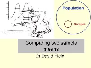
Hypothesis TestingPopulation Means: Large Samples Is there a difference in the mean amount to residential real estate sold by male agents and female agents in south Florida? • Let’s select random samples from 2 populations. We wish to investigate if these populations have the same mean • Want to determine whether the samples are from the same or equal populations • If the 2 populations are the same, we would expect the difference between the 2 sample means to be zero • 2 assumptions needed: • Both samples are at least 30 • The samples are from independent populations
Example • A financial analyst wants to compare the turnover rates, in percent, for shares of oil-related stocks versus other stocks, such as GE and IBM. She selected 32 oil-related stocks and 49 other stocks. The mean turnover rate of oil-related stocks is 31.4 percent and the standard deviation 5.1 percent. For the other stocks, the mean rate was computed to be 34.9 percent and the standard deviation 6.7 percent. Is there a significant difference in the turnover rates of the two types of stock? Use the .01 significance level.
Hypothesis TestingPopulation Means: Small Samples Is the mean salary of nurses larger than that of school teachers? • The sample size is less than 30 • ‘Small sample test of means’ • The 2 sample variances are pooled to estimate population variance; weighted mean • The weights are the degrees of freedom that each sample provides • Assumptions: • 1. The sampled populations follow the normal distribution • 2. The two samples are from independent populations • 3. The standard deviations of the two populations are equal
Example • A recent study compared the time spent together by single- and dual-earner couples. According to the records kept by the wives during the study, the mean amount of time spent together watching television among the single-earner couples was 61 minutes per day, with a standard deviation of 15.5 minutes. For the dual-earner couples, the mean number of minutes spent watching television was 48.4 minutes, with a standard deviation of 18.1 minutes. At the .01 significance level, can we conclude that the single-earner couples on average spend more time watching television together? There were 15 single-earner and 12 dual-earner couples studied.