Monte Carlo Simulation
Monte Carlo Simulation. Wednesday, 9/11/2002. Ensemble sampling Markov Chain Metropolis Sampling. Stochastic simulations consider particle interactions. Deterministic vs. Stochastic. Newton’s equation of motion. F = m a. Random Walk. Brownian motion. n = 200 s = .02

Monte Carlo Simulation
E N D
Presentation Transcript
Monte Carlo Simulation Wednesday, 9/11/2002 • Ensemble sampling • Markov Chain • Metropolis Sampling Stochastic simulations consider particle interactions.
Deterministic vs. Stochastic Newton’s equation of motion F = ma Random Walk
Brownian motion n = 200 s = .02 x = rand(n,1)-0.5; y = rand(n,1)-0.5; h = plot(x,y,'.'); axis([-2 2 -2 2]) axis square grid off set(h,'EraseMode','xor','MarkerSize',18) while 1 drawnow x = x + s*randn(n,1); y = y + s*randn(n,1); set(h,'XData',x,'YData',y) end Animations
Lennard-Jones Potential force potential
Replace the time average with ensemble average An ensemble is a collection of systems. The probability for a system in state s is Ps. If you average the velocity of one molecule of the air in your room, as it collides from one molecule to the next, that average comes out the same as for all molecules in the room at one instant.
Thought experiment Let’s pretend that our universe really is replicated over and over -- that our world is just one realization along with all the others. We're formed in a thousand undramatic day-by-day choices. Parallel universes ensembles
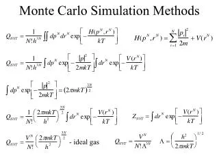
Canonical Ensemble Fixed number of atoms, system energy, and system volume. Partition function
Finite number of microstates Importance sampling
Metropolis Sampling I 1. Current configuration: C(n) 2. Generate a trial configuration by selecting an atom at random and move it. 3. Calculate the change in energy for the trial configuration, DU.
Metropolis Sampling II If DU < 0, accept the move, so that the trial configuration becomes the (n+1) configuration, C(n+1). If DU >= 0, generate a random number r between 0 and 1; If r <= exp( -DU/kBT ), accept the move, C(n+1) = C(t); If r > exp( -DU/kBT ), reject the trial move. C(n+1) = C(n). A sequence of configurations can be generated by using the above steps repeatedly. Properties from the system can be obtained by simply averaging the properties of a large number of these configurations.
Markov Chain A sequence X1, X2, …, of random variable is called Markov if, for any n, i.e., if the conditional distribution F of Xn assuming Xn-1, Xn-2, …, X1 equals the conditional distribution F of Xn assuming of only Xn-1.
Markov Process Dart hit-or-miss Random Walk (RW) Self-Avoiding Walk (SAW) Growing Self-Avoiding Walk (GSAW) Diffusion Limited Aggregation http://apricot.polyu.edu.hk/~lam/dla/dla.html

