Download
1 / 8
80 likes | 111 Views
Learn about joint distributions of discrete and continuous random variables, marginal distributions, independence tests, and propagation. Slides based on the book "A Modern Introduction to Probability and Statistics."

E N D
MATH 3033 based onDekking et al. A Modern Introduction to Probability and Statistics. 2007Slides by Michael MauriziFormat by Tim Birbeck Instructor Longin Jan Latecki C9: Joint Distributions and Independence
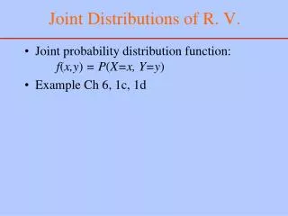
9.1 – Joint Distributions of Discrete Random Variables • Joint Distribution: the combined distribution of two or more random variables defined on the same sample space Ω • Joint Distribution of two discrete random variables:The joint distribution of two discrete random variables X and Y can be obtained by using the probabilities of all possible values of the pair (X,Y) Joint Probability Mass function p of two discrete random variables X and Y: Joint Distribution function F of two random variables X and Y: Can be thought of as the sum of the elements in box it makes with the upper-left corner.
9.1 – Joint Distributions of Discrete Random Variables • Marginal Distribution: Obtained by adding up the rows or columns of a joint probability mass function table. Literally written in the margins. Example: Joint Distribution of S and M. S = The sum of two dice, M = The maximum of two dice. Marginal distribution function of X: Marginal distribution function of Y:
9.2 – Joint Distributions of Continuous Random Variables • Joint Continuous Distribution: Like an ordinary continuous random variable, only works for a range of values. There must exist a function f that fulfills the following properties for there to be a joint continuous distribution:
9.2 – Joint Distributions of Continuous Random Variables Joint distribution function: F(a,b) can be constructed given f(x,y), and vice versa Marginal probability density function: You need to integrate out the unwanted random variable to get the marginal distribution.
9.3 – More than Two Random Variables Assuming we have n random variables X1, X2, X3, … Xn. We can get the joint distribution function and the joint probability mass functions.
9.4 – Independent Random Variables Tests for Independence: Two random variables X and Y are independent if and only if every event involving X is independent of every event involving Y. This also applies to joint distributions using more than two random variables.
9.5 – Propagation of Independence Independence after a change of variable: If a function is applied to several independent random variables, the new resulting random variables will also be independent.