Understanding NURBS: The Evolution from Spline to Non-Uniform Rational B-Splines
300 likes | 432 Views
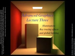
This lecture, presented by Alex Benton at the University of Cambridge, explores the history and development of splines, particularly focusing on NURBS (Non-Uniform Rational B-Splines). The term "spline" originates from shipbuilding, where wooden strips were used as flexible curves. The lecture covers the mathematical foundations of Bezier curves, their applications in industries like automotive and design, and how NURBS generalize these concepts, allowing for greater control over curve shapes and continuity. It emphasizes smooth curves' critical role in perceived quality.

Understanding NURBS: The Evolution from Spline to Non-Uniform Rational B-Splines
E N D
Presentation Transcript
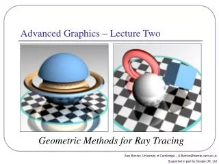
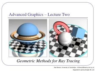
Advanced GraphicsLecture Five Revenge of the NURBS Alex Benton, University of Cambridge – A.Benton@damtp.cam.ac.uk Supported in part by Google UK, Ltd
History • The term ‘spline’ comes from the shipbuilding industry: long, thin strips of wood or metal would be bent and held in place by heavy ‘ducks’, lead weights which acted as control points of the curve. • Wooden splines can be described by Cn-continuous Hermite polynomials which interpolate n+1 control points. Top: Fig 3, P.7, Bray and Spectre, Planking and Fastening, WoodenBoat Pub (1996) Bottom: http://www.pranos.com/boatsofwood/lofting%20ducks/lofting_ducks.htm
History • Curves which must have n+1 control points are hard to work with. (n+1)x(m+1) patches are even moreso. • But continuity—smooth curves—is essential to the perception of quality of manufacture. Especially in cars, and some Apple products. • Splines were generalized in the 1960s by Bezier (Renault), de Casteljau (Citroen), de Boor (GM).
Beziers—a quick review • A Bezier cubic is a function P(t) defined by four control points: • P0 and P3 are the endpoints of the curve; P1 and P2 define the other two corners of the bounding trapezoid. • The curve fits entirely within the bounding trapezoid. P1 P2 P0 P3
Joining Bezier splines • To join two Bezier splines with C0 continuity, set P3=Q0. • To join two Bezier splines with C1 continuity, require C0 and make the tangent vectors equal: set P3=Q0 and P3-P2=Q1-Q0. Q1 Q0 P3 P2
Joining Bezier patches • This works for Bezier patches as well: to join two patches with C1 continuity at an edge, ensure that their control points and tangent vectors on that edge are equal. • NURBS patches arejoined in exactly thesame way.
Beziers • Cubics, of course, are just one example of Bezier splines: Linear: P(t) = (1-t)P0 + tP1 Quadratic: P(t) = (1-t)2P0 + 2t(1-t)P1 + t2P2 Cubic: P(t) = (1-t)3P0 + 3t(1-t)2P1 + 3t2(1-t)P2 + t3P3 ... General: “n choose v” = n! / i!(n-i)!
Beziers P1 (1-t)P1+tP2 • Thinking about Beziers • Linear interpolations • The linear Bezier is a linear interpolation between two points. • The quadratic Bezier can be seen as a linear interpolation between two lines: P(t) = (1-t) ((1-t)P0+tP1) + (t) ((1-t)P1+tP2) • The cubic is a linear interpolation between linear interpolations between linear interpolations… etc. • Another way to see Beziers is as a weighted average between the control points. (1-t)P0+tP1 P2 P(t) P0
Bernstein polynomials P(t) = (1-t)3P0 + 3t(1-t)2P1 + 3t2(1-t)P2 + t3P3 • The four control functions are the four Bernstein polynomials for n=3. • General form: • Bernstein polynomials in 0 ≤ t ≤ 1 always sum to 1:
We can parameterize this chain over t by saying that instead of going from 0 to 1, t moves smoothly through the intervals [0,1,2,3] The curve C(t) would be: C(t) = P(t) • ((0 ≤ t <1) ? 1 : 0) + Q(t-1) • ((1 ≤ t <2) ? 1 : 0) + R(t-2) • ((2 ≤ t <3) ? 1 : 0) [0,1,2,3] is, in a way, a type of knot vector. 0, 1, 2, and 3 are the knots. This is not strictly true, but the idea is right: knots define intervals. Consider a chain of splines with many control points… P = {P0, P1, P2, P3} Q = {Q0, Q1, Q2, Q3} R = {R0, R1, R2, R3} …with C1 continuity… P3=Q0, P2-P3=Q0-Q1 Q3=R0, Q2-Q3=R0-R1 Parameterizing a chain of Beziers Q1 Q2 Q0 Q3 P3 R0 P2 R1
NURBS • NURBS (“Non-Uniform Rational B-Splines”) are a generalization of Beziers. • NU: Non-Uniform. The control points don’t have to be weighted equally. • R: Rational. The spline may be defined by rational polynomials (homogeneous coordinates.) • BS: B-Spline. A chained series of Bezier splines with controllable degree.
B-Splines • A Bezier cubic is a polynomial of degree three: it must have four control points per spline, it must begin at the first and end at the fourth, and it assumes that all four control points are equally important. • Beziers are actually a type of B-spline. B-splines are a piecewise parameterization of Beziers that supports an arbitrary number of control points and lets you specify the degree of the polynomial which interpolates them.
B-Splines • We’ll build our definition of a B-spline from: • n+1, the number of control functions • k, the degree of the curve • {P0…Pn}, a list of n+1control points • [t0,t1,…,tk+n+1], a knot vector of parameter values • n intervals → n+1 control points • k is the degree of the curve, so k+1 is the number of control points which influence a single interval. k must be at least 1 (two control points linked by each linear line segments) and no more than n (the number of intervals.) • There are k+n+2 knots, and ti ≤ ti+1 for all ti.
B-Splines • The equation for a B-spline is • Ni,k(t) is the basis function of control point Pi. Ni,k(t) is defined recursively:
B-Splines t0 t1 t2 t3 t4 … N1,0(t) N2,0(t) N3,0(t) … N0,0(t) N1,1(t) N2,1(t) … N0,1(t) N1,2(t) N0,2(t) … N0,3(t) …
B-Splines 0 1 1 2 2 3 3 4 4 5 N0,0(t) N1,0(t) N2,0(t) N3,0(t) N3,0(t) Knot vector = {0,1,2,3,4,5}, k = 0
B-Splines N0,1(t) N1,1(t) N2,1(t) N3,1(t) Knot vector = {0,1,2,3,4,5}, k = 1
B-Splines N0,2(t) N1,2(t) N2,2(t) Knot vector = {0,1,2,3,4,5}, k = 2
B-Splines At k=1 the function is piecewiselinear, depends on P0,P1,P2,P3, and is fully defined on [t1,t4). At k=2 the function is piecewisequadratic, depends on P0,P1,P2, and is fully defined on [t2,t3). Each degree-k control function depends on k+1 knot values, so Ni,k depends on ti through ti+k, inclusive. So six knots → five discontinuous functions → four piecewise linear interpolations → three quadratics, interpolating three control points. n+1=3 control points, k=2 degree, n+1+k+1=6 knots. Knot vector = {0,1,2,3,4,5}
Non-Uniform B-Splines • The knot vector {0,1,2,3,4,5} is uniform: ti+1-ti = ti+2-ti+1 ti. • Varying the size of an interval changes the parametric-space distribution of the weights assigned to the control functions. • Repeating a knot value reduces the continuity of the curve in the affected span by one degree. • Repeating a knot k+1 times will lead to a control function being influenced only by that knot value; the spline will pass through the corresponding control point with C0 continuity.
Open vs Closed • A knot vector which repeats its first and last knot values k+1 times is called closed, otherwise open. • Repeating the knots k+1 times is the only way to force the curve to pass through the first or last control point. • Without this, the functions N0,kand Nn,kwhich weight P0and Pn would still be ‘ramping up’ and not yet equal to one at the first and last ti.
Open vs Closed • Two examples you may recognize: • k=2, n+1=3 control points, knots={0,0,0,1,1,1} • k=3, n+1=4 control points, knots={0,0,0,0,1,1,1,1}
Non-Uniform Rational B-Splines • Repeating knot values is a clumsy way to control the curve’s proximity to the control point. • We want to be able to slide the curve nearer or farther without losing continuity or introducing new control points. • The solution: homogeneous coordinates. • Associate a ‘weight’ with each control point: ωi.
Non-Uniform Rational B-Splines • Recall: [x, y, z, ω]H→ [x / ω, y / ω, z / ω] • Or: [x, y, z,1] → [xω, yω, zω, ω]H • The control point Pi=(xi, yi, zi) becomes the homogeneous control point PiH =(xiωi, yiωi, ziωi) • A NURBS in homogeneous coordinates is:
Non-Uniform Rational B-Splines • To convert from homogeneous coords to normal coordinates:
Non-Uniform Rational B-Splines • A piecewise rational curve is thus defined by: with supporting rational basis functions: • This is essentially an average re-weighted by the ω’s. • Such a curve can be made to pass arbitrarily far or near to a control point by changing the corresponding weight.
Tensor products for surfaces • The tensor product of two vectors is a matrix. • Can also take the tensor of two polynomials.
NURBS surfaces • The tensor product of the polynomial coefficients of two NURBS splines is a matrix of polynomial coefficients. • If curve A has degree k and n+1 control points and curve B has degree j and m+1 control points then A⊗B is an (n+1)x(m+1) matrix of polynomials of degree max(j,k). • So all you need is (n+1)(m+1) control points and you’ve got a rectangular surface patch! • This approach generalizes to triangles and arbitrary n-gons.
References • Les Piegl and Wayne Tiller, The NURBS Book, Springer (1997) • Alan Watt, 3D Computer Graphics, Addison Wesley (2000) • G. Farin, J. Hoschek, M.-S. Kim, Handbook of Computer Aided Geometric Design, North-Holland (2002) Really good book!