4. The Grand Canonical Ensemble

1. 4. The Grand Canonical Ensemble Equilibrium between a System & a Particle-Energy Reservoir A System in the Grand Canonical Ensemble Physical Significance of Various Statistical Quantities Examples Density & Energy Fluctuations in the Grand Canonical Ensemble: Correspondence with Other Ensembles Thermodynamic Phase Diagrams Phase Equilibrium & the Clausius-Clapeyron Equation

2. 4.1. Equilibrium between a System & a Particle-Energy Reservoir System A immersed in particle-energy reservoir A. A in microstate with Nr & Es with Using  

3. A, A in eqm   

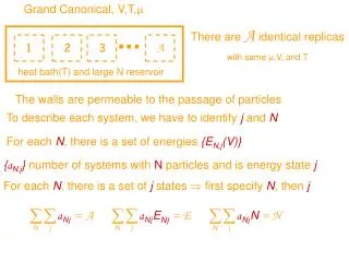
4. 4.2. A System in the Grand Canonical Ensemble Consider ensemble of N identical systems sharing particles & energy Let nr,s= # of systems with Nr & Es , then Let W {nr,s } = # of ways to realize a given set of distribution { nr,s} .  Method of Most Probable Values : Let {nr,s* } = most probable set of distribution, i.e., 

5. Method of Mean Values : (X) means sum includes only terms that satisfy constraint on X. Saddle point method  For a given the parameters & are determined from Classical mech (Gibb –corrected ):

6. 4.3. Physical Significance of Various Statistical Quantities The q-potential is defined as dEs caused by dV.  

7.     Euler’s eq. 

8. Fugacity   Variable dependence : Grand partition function Note: Zis much easier to evaluate than Z, especially for quantum statistics and/or interacting systems.

9. Grand Potential Approach Let F be the thermodynamic potential related to Z. Grand potential Particle, heat reservoir  Suggestion from canonical ensemble :  

10.   

11. Grand Potential See Reichl, §2.F.5. Grand potential : Caution :   Prob 4.2

12. Using we have 

13. 4.4. Examples Classical Ideal Gas : N ! = Correction for Indistinguishableness Freely moving particles  

15.    n = 3/2 : nonrelativistic gas. n = 3: relativistic gas. Find A & S as functions of (T,V,N) yourself.

16. Non-Interacting, Localized Particles Non-Interacting, Localized Particles (distinguishable particles : model for solid ) : Particles localized   for or

17.   

18. Quantum 1-D oscillators: See §3.8 Classical limit : Consider a substance in vapor-solid phase equilibrium inside a closed vessel .  i.e., Phase equilibrium 

19. For ideal gas vapor : If   For a monatomic gas :  From §3.5 Einstein model : solid ~ 3-D oscillators of same  

20.  ( e / kT added by hand to account for the difference between binding energies of the solid & gas phases. ) At phase equilibrium: Pure vapor :  Tc = characteristic T Solid phase appears :  or Since f /  e / kT increases with T, this means Mathematica

21. 4.5. Density & Energy Fluctuations in the Grand Canonical Ensemble: Correspondence with Other Ensembles with  see §3.6 In general

22. Particle density :  Particle volume :  1st law :  Euler’ s equation :   T= isothermal compressibility

23. Relative root mean square of n ~ 0 in the thermodynamic limit for finite T  , = critical exponents d = dimension of system At phase transition : Experiment on liquid-vapor transition : root mean square of n critical opalescence  Grand canonical  canonical ensemble

24. Energy Fluctuations  Caution : N = N( P,T ) 

25.  §3.6:  

26. 4.6. Thermodynamic Phase Diagrams Phase diagram: Thermodynamic functions are analytic within a single phase, non-analytic on phase boundaries. Ar Tt = 83.8 K Pt = 68.9 kPa TC = 150.7 K PC = 4.86 MPa supercritical fluid Co-existence lines : S-L L-V S-V Liquid Solid Vapor A = Triple point C = Critical point

27. Ar Triple point Tt = 83.8 K Pt = 68.9 kPa Critical point TC = 150.7 K PC = 4.86 MPa supercritical fluid Co-existence lines : S-L L-V S-V

28. supercritical fluid Liquid Solid Vapor supercritical fluid Co-existence lines : S-L L-V S-V

29. 4He (BE stat) : Critical point TC = 5.19 K PC = 227 kPa T = 2.18 K PS = 2.5MPa 4He 3He (FD stat) : Critical point TC = 3.35 K PC = 227 kPa PS = 30MPa Superfluid characteristics (BEC) : Viscosity = 0. Quantized flow. Propagating heat modes. Macroscopic quantum coherence. Superfluid below 10 mK due to BCS p-wave pairing.

30. 4.7. Phase Equilibrium & the Clausius-Clapeyron Equation Gibbs free energy =  ( P,T ) = chemical potential Consider vessel containing Nmolecules at constant T & P. Let there be 2 phases initially: vapor (A) & liquid (B).  For a given T & P : See Reichl §2.F At equilibrium, G is a minimum  for spontaneous changes

31. T, P fixed  for spontaneous changes  At coexistence so that NAcan assume any value between 0 & N. Actual NA assumed is determined by U ( via latent heat of vaporization ). Coexistence curve in P-T plane is given by where   

32.  Clausius-Clapeyron eq. ( for 1st order transitions ) Latent heat per particle. Prob. 4.11, 4.14-6. At triple point are related  Slopes since Prob. 4.17.