Download
1 / 42
850 likes | 3.59k Views
Lecture 11: The Grand Canonical Ensemble. Schroeder Ch. 7.1-7.3 Gould and Tobochnik 6.3-6.5, 6.8. Outline. Derivation of the Gibbs distribution Grand partition function Bosons and fermions Degenerate Fermi gases White dwarfs and neutron stars Density of states Sommerfeld expansion

E N D
Lecture 11: The Grand Canonical Ensemble Schroeder Ch. 7.1-7.3 Gould and Tobochnik 6.3-6.5, 6.8
Outline • Derivation of the Gibbs distribution • Grand partition function • Bosons and fermions • Degenerate Fermi gases • White dwarfs and neutron stars • Density of states • Sommerfeld expansion • Semiconductors
Introduction • We have already described the canonical ensemble, which is defined as a collection of closed systems. • If we relax the condition that no matter is exchanged between the system and its reservoir, we obtain the grand canonical ensemble. • In this ensemble, the systems are all in thermal equilibrium with a reservoir at some fixed temperature, but they are also able to exchange particles with this reservoir.
Derivation of Gibbs Distribution • What is the probability of finding a member of the ensemble in a given state with energy and containing particles? • Consider a system in thermal and diffusive contact with a reservoir, , whose temperature and chemical potential are effectively constant. • If has energy and particles, then the total number of states available to the combined system is
Derivation of Gibbs Distribution • Since the combined system belongs to a microcanonical ensemble, the probability of finding our system with energy and particles is given by • Since the reservoir is very large compared with our system, then and
Derivation of Gibbs Distribution • Expanding in a Taylor series about gives • Writing the above expression in terms of temperature and chemical potential gives
Derivation of the Gibbs Distribution • Since the combined system is in the microcanonical ensemble, then the probability of finding in any one state of energy and particles is given by • Each of the exponential factors is called a Gibbs factor • If we define the constant as , then for any state , the probability is given by • This is the Gibbs distribution and it characterizes the grand canonical ensemble
Grand Partition Function • The quantity is called the grand partition function. • By requiring that the sum of the probabilities of all states to equal 1, it can be shown that
Example • Consider a system consisting of a single hydrogen atom, which has two possible states: • Unoccupied (i.e. no electron present) • Occupied (one electron present in the ground state) • Q: What is the ratio of the probabilities of these two states?
Example • If we neglect the spin states of the electron and the excited states of the hydrogen atom, this system has just two states • Unoccupied: • Occupied: • The ratio of the probabilities of these two states s given by
Example • If we treat the electrons as a monatomic ideal gas, then the chemical potential for electrons is given by • Therefore, we have
Example • Taking electron spin into account, the hydrogen atom now has two occupied states, each with the same energy, so the ratio of unoccupied to occupied atoms is • Now, a free electron has two degenerate states so the chemical potential of the electron gas is • Therefore, we have
Thermodynamics in the Grand Canonical Ensemble • It can be shown that all the thermodynamic functions can be expressed in terms of the grand partition function and its derivatives. • The average internal energy is • The average number of particles is • The generalized forces are • The entropy is given by
Grand Potential • Recall that in the canonical ensemble, there is a relationship between the Helmholtz free energy and the partition function: . • Using an analogous argument, we can derive the grand potential: • The grand potential is the maximum amount of energy available to do external work for a system in contact with both a heat and a particle reservoir.
Bosons and Fermions • The most important application of Gibbs factors is to quantum statistics: the study of dense systems in which 2+ identical particles have a probability of occupying the same single-particle state. • Particles that can share a state with another of the same species are called bosons. • Examples include photons, helium-4 atoms, etc. • Particles that cannot share a state with another of the same species are called fermions. • Examples include protons, neutrons, neutrinos, etc.
Bosons and Fermions • Because individual particles have wave-like properties, the state of a particle can be described by a wavefunction • The indistinguishability of quantum-mechanical particles implies that • Observations show that both signs are possible for quantum-mechanical particles For bosons For fermions
Bosons and Fermions • Suppose that the two-particle wavefunction can be decomposed into a product of single-particle wavefunctions • For bosons, this equation guarantees that will be symmetric under interchange of and . • For fermions, this equation guarantees that . • The rule that two identical fermions cannot occupy the same state is called the Pauli exclusion principle • Pauli also demonstrated that all particles with integer spins are bosons, whereas all particles with half-integer spin are fermions.
Bosons and Fermions • When , the chance of any two particles occupying the same state is negligible. • For an ideal gas, the chance of any two particles occupying the same state is negligible only if . • There are a number of systems that violate this condition • Neutron star • Liquid helium • Electrons in metals • Photons
Fermi-Dirac Distribution • Consider a single-particle state of a system whose energy when occupied by a single particle is . The probability of the state being occupied by particles is • If the particles in question are fermions, then can only be 0 or 1, which implies that • The average number of particles in the state (also called the occupancy of the state) is given by • This distribution is called the Fermi-Dirac distribution
Fermi-Dirac Distribution • The Fermi-Dirac distribution goes to zero when and goes to 1 when . • At very low temperature, fermions will distribute themselves in the energy levels below the chemical potential and all the levels above are empty. • As the temperature rises, energy levels above the chemical potential begin to be occupied.
Degenerate Fermi Gases • As an application of the Fermi-Dirac distribution, let’s examine degenerate Fermi gases. • Examples of degenerate Fermi gases are • Conduction electrons in a metal • Electrons in a white dwarf star • Neutrons in a neutron star • Let’s first consider the properties of an low-temperature electron gas.
Low-Temperature Electron Gas • At , the Fermi-Dirac distribution becomes a step function in which all single-particle states with energy less than are occupied, while all states with energy greater than are unoccupied. • In this context, is also called the Fermi energy • When a gas of fermions is so cold that nearly all states below are occupied, it is said to be degenerate. • It can be shown that the Fermi energy is given by
Low-Temperature Electron Gas • Thus, the Fermi energy is the highest energy of all the electrons. • To calculate the total energy of all the electrons, we can add up the energies of the electrons in all occupied states. • It can be shown that the total energy is
Low-Temperature Electron Gas • Therefore, the average energy of the electrons is 3/5 the Fermi energy. • The temperature that a Fermi gas would have to have in order for is called the Fermi temperature. • The pressure of a degenerate electron gas (also called the degeneracy pressure) is given by • The degeneracy pressure is what keeps matter from collapsing under the electrostatic forces that attract electrons and protons.
White Dwarfs and Neutron Stars • A star that has consumed all its nuclear fuel will undergo gravitational collapse, but may end up in a stable state as a white dwarf or a neutron star. • This occurs when the mass that remains in the core after the outer layers are blown away doesnot exceed a particular limit, called the Chandrashekar limit. • Stars that succeed in forming such stable remnants owe their existence to the high degeneracy pressure exerted by electrons (for white dwarfs) and neutrons (for neutron stars).
White Dwarf Stars • A white dwarf star can be considered as a degenerate electron gas. • The nuclei present within the white dwarf balances the charge and provides the gravitational attraction that holds the star together. • The total kinetic energy of the degenerate electrons is given by the Fermi energy
White Dwarf Stars • If we assume that the star contains one proton and one neutron for each electron, then and thus we have • The Fermi energy and Fermi temperature for the white dwarf star is given by • Here, is the equilibrium radius of a white dwarf star, which can be determined by finding the minimum of the total energy
White Dwarf Stars • It can be shown that the gravitational potential energy of a white dwarf is given by • The total energy of a white dwarf can be given by • The equilibrium radius of a white dwarf is determined by the minimum of the total energy • For a one solar mass white dwarf, and thus, the Fermi energy and the Fermi temperature for the white dwarf star is given by
Neutron Stars • A neutron star is made entirely of neutrons and is supported against gravitational collapse by degenerate neutron pressure. • The total kinetic energy of the degenerate electrons is given by the Fermi energy • Thus, the kinetic energy comes from the neutrons, and the number of these is simply . Therefore, we have • The Fermi energy and the Fermi temperature for the neutron star is given by
Neutron Stars • The total energy of a neutron star can be given by • The equilibrium radius of a white dwarf is determined by the minimum of the total energy • For a one solar mass white dwarf, and thus, the Fermi energy and the Fermi temperature for the neutron star is given by
Density of States • One property of a Fermi gas that we cannot calculate using the approximation is the heat capacity. • Therefore, we must examine the Fermi gas at small nonzero temperatures • To better visualize – and quantify – the behavior of a Fermi gas at small temperatures, we will introduce a new concept called the density of states.
Density of States • Using a suitable change of variables, it can be shown that the energy integral for a Fermi gas at zero temperature becomes • The quantity in square brackets is the number of single particle states per unit energy, also known as the density of states. • Using the density of states, we can obtain the total number of electrons at zero temperature
Density of States • For nonzero temperature, the total number and energy of electrons can be determined as follows • Note that the chemical potential is the point where the probability of being occupied is exactly ½. • In the limit , we can use the Sommerfeld expansion to evaluate the above integrals.
Sommerfeld Expansion • Performing integration by parts gives • The boundary term vanishes at both limits and using a suitable change in variables, we have
Sommerfeld Expansion • We can make two approximations • Extend the lower limit to • Expand in a Taylor series about the point • With these approximations, we have • This integral can be performed giving
Sommerfeld Expansion • Solving for gives • Performing the same expansion for the total energy gives • From this result, we can easily calculate the heat capacity
Electrons in Metals • Atoms in a metal are closely packed, which causes their outer shell electrons to break away from the parent atoms and move freely through the solid. • The set of electron energy levels for which they are more or less free to move in the solid is called the conduction band. • Energy levels below the conduction band form the valence band and electrons at energies below that are strongly bound to the atoms. • The work function, , is the energy that an electron must acquire to escape the metal.
Conductors and Insulators • In a conductor, the Fermi energy lies within one of the bands, whereas in an insulator, the Fermi energy lies within a gap. • Therefore, at , the band below the gap is completely occupied while the band above the gap is unoccupied. • Because there are no empty states close in energy to those that are occupied, the electrons are “stuck in place” and the material does not conduct electricity.
Semiconductors • A semiconductor is an insulator in which the gap is narrow enough for a few electrons to jump across it at room temperature. • The figure below shows the density of states in the vicinity of the Fermi energy for an idealized semiconductor.
Semiconductors • As an approximation, let’s model the density of states near the bottom of the conduction band using the same function as for a free Fermi gas with an appropriate zero point. • Let’s model the density of states near the top of the valence band as a mirror image of this model. • In this approximation, the chemical potential must always lie precisely in the middle of the gap, regardless of the temperature.
Semiconductors • The number of electrons in the conduction band is given by • If the width of the gap is much greater than , then we can approximate the above integral as • After a suitable change in variables, this integral can be evaluated to give
Semiconductors • The above result indicates that a pure semiconductor will conduct much better at higher temperature because there are much more electrons in the conduction band. • Moreover, in order to produce an insulator, the gap would have to become significantly wider.