Download
1 / 20
210 likes | 346 Views
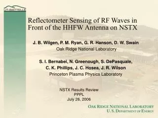
Reflectometer Measurements of the Plasma Edge in front of the HHFW antennas. John Wilgen, David Swain, Greg Hanson, Phil Ryan Oak Ridge National Laboratory Randy Wilson et al. Princeton Plasma Physics Laboratory NSTX Results Review Meeting PPPL September 9 – 11, 2002.

E N D
Reflectometer Measurements of the Plasma Edge in front of the HHFW antennas • John Wilgen, David Swain, Greg Hanson, Phil Ryan • Oak Ridge National Laboratory • Randy Wilson et al. • Princeton Plasma Physics Laboratory • NSTX Results Review Meeting • PPPL • September 9 – 11, 2002
HHFW Broadband Microwave Reflectometer • Purpose:Measure the edge density profile directly in front of the HHFW antenna, primarily in the scrape-off layer in the gap between the outermost flux surface and the antenna • Topics to be covered: • Reflectometer access (thru HHFW antenna) • Measurement capability: Profiles & Fluctuations • Current Status of Data Analysis • Examples of profile data obtained for: • H-mode conditions • Co-CD in Helium Plasma • When outer gap --> 0 • Example of fluctuation data • Summary
HHFW Reflectometer Access Located Between 2nd and 3rd Straps of the HHFW antenna Location of ORNL microwave reflectometer launchers used for edge density profile measurements
Cylindrical Waveguide Antennas - HHFW Reflectometer • Antennas are recessed 2.5 cm behind BN tiles (& Faraday screen) • Linear polarized launch couples to X-mode propagation in plasma • Launched polarization externally adjustable to match the pitch angle of the magnetic field (typically 35 degrees off vertical) 1.5” OD Cylindrical Waveguide Antenna
Operational modes for HHFW ReflectometerCan switch between fluctuation & profile modes remotely, between shots • Profile Measuring Mode • Sweep time: 100 msec • Frequency range: 5.74 to 26.8 GHz • X-mode polarization (sweep starts below cyclotron frequency) • Density range: 0.05 to 6.0 x 1012 cm-3 • Due to low starting density, profile reconstruction normally begins at the leading edge of the HHFW antenna • Analyzed profile data is written to the MDSPlus tree • Data taken in 200 ms window; start time can be changed shot-to-shot • Fluctuation Measuring Mode • Fluctuation mode - dwell at 2 fixed frequencies, switching every 5 ms • Standard Dwell Frequencies: 14.2 & 20.4 GHz (but can be changed) • Cutoff densities: 1.2 & 3.5 x 1012 cm-3 • Fluctuation data was collected for 32 shots from 6 different days • Analyzed fluctuation data is not written to the tree
Status of HHFW Reflectometer Data Analysis • Data Analysis - Reconstruction of Edge Density Profiles • Automated profile reconstruction for entire shot • Uses accelerated reconstruction to get “quick and dirty” profiles • Caution: Not all of the profiles are credible • Up to 1000 profiles written to the tree for each shot • Also write “averaged” density profiles (9-sweep averages, 1.8 ms) • Analysis code has been run on between-shots basis • Status of the Profile Data Analysis • Reflectometer data was collected for > 1200 shots; most are on HHFW run days, but also have other data (4/1-5, 4/15-24, 5/8-24, 6/10-14) • We have some earlier data (2/25-26) that can also be analyzed • All since107502 (4/3/02) have been analyzed & written to the tree • Now have > 1.2 million profiles available (not all are credible) • Next Step: Algorithms for assigning confidence factor to each profile
Routines to access the data are available • Accessing Edge Density Profile Data from the Tree: • Option 1: Obtain data from tree as structure a la TS routines • Use NSTX$:[ornlrefl.source]getreflanalyzeddata.pro • getreflanalyzeddata,shotnumber,results,error_flag • results - structure with analyzed data, contains: • calshot - LONG - calibration shot used in analysis • version - TEXT - version of code used in analysis • analysisdata - TEXT - analysis date and time • comment - TEXT - comment on analysis, data,.... • fvector -FLOAT[fdim] - vector of frequencies for phase output • rvector - FLOAT[rdim] - vector of radius for density output • tvector - FLOAT[nsweeps] - starting times for each reflectometer sweep • density - FLOAT[rdim,nsweeps] - density(rvector,tvector) • phase - FLOAT[fdim,nsweeps] - phase(fvector,tvector) • quality - FLOAT[fdim,nsweeps] - quality of data (fvector,tvector) • avgdensity = FLOAT[rdim,avgdim] - density averaged over 9 sweeps • avgtvector = FLOAT[avgdim] - time of average density curves • error_flag = 0 if data returned OK, = 1 if not
Plotting routine for the reflectometer data is also available • Option 2: Use analysis code to view various plots of data • Set default area to NSTX$:[ornlrefl.source] • REFLVIEWwill start display program (widget-based, needs X-windows) • Set the shot you want, and (optional) the time you want • You can plot: • Multiple plots of groups of 9 successive sweeps of phase(frequency) or density(R) • Averaged density profiles for entire shot (200 ms) • Big plot of phase and density for a specific time (suitable for framing) • Contour plot showing averaged profile evolution vs time • Bugs exist – let us know when you fine one! (swaindw@ornl.gov)
Analysis Code Display: Phase Data & Reconstructed Profiles162 density profiles for 108317, starting at 80 msec Density (1019 m-3) Radius (m) Each box contains data from 9 consecutive sweeps over 1.8 ms period Heavy black line is the average of the nine sweeps (used in contour plot) Can also plot reflectometer phase data in similar manner
Analysis Code Display: Average Density Profiles63 averaged profiles for shot 107443, starting at 180 ms Starting off with L-mode plasma conditions H-mode transition occurs midway thru this frame All H-mode Following the H-mode transition, > density is depleted in scrape-off layer > fluctuations are greatly reduced > consecutive sweeps yield identical profiles > the reflectometer works!!!
Analysis Code: Contour Plot of Average density vs. timeFluctuations are reduced at H-mode transition (≈ 237 ms)! 10 Density Contours (x1019 m-3) Shot 107443 8 Profiles tend to follow the outer gap Distance From HHFW Antenna (cm) 6 4 2 H-mode transition 0 180 200 220 240 260 280 300 Time (ms)
Credibility of Reflectometer Density Profiles • L-mode reflectometer data is often problematic, phase data is often phase scrambled with resulting fringe skips • Nevertheless, averaged profiles are useful in revealing trends in the time evolution of the density profile in the scrapeoff layer • Three Cases Where Reflectometer Data is Exceptional • Certain H-mode transitions (like shot 107443) • Density is depleted in the scrape-off layer • Fluctuations are greatly reduced • As many as 20 consecutive sweeps yield identical profiles • Co-current drive phasing in He plasmas • Fluctuations are reduced relative to CCD phasing • Certain shots where the Outer Gap --> 0 (like shot 107524) • Profiles are typically very steep (good for EBW emission) • Fluctuations are suppressed
Profiles Show Reduced Fluctuations After H-mode Transition15 consecutive sweeps in each frame (m) (ms)
Comparison of Co vs Counter-CD Phasing in Helium PlasmaFluctuations in Averaged Profiles are Clearly Reduced for Co-CD Phasing ! HHFW Counter-CD Phasing HHFW Co-CD Phasing Shot 108571 Shot 108565 400 300 350 400 250 300 350 250 Time (msec) Time (msec) This difference was very consistent throughout the entire day (5/21/02)
Density Contours Shift Outward When Gap--> 0Profiles becomes very steep, fluctuations are suppressed ! Density Contours (x1019 m-3) Shot 107524 Show Profiles 8 Distance From HHFW Antenna (cm) 6 4 2 0 150 200 250 300 350 400 Time (ms)
Fluctuations are Suppressed when Outer Gap ---> 025 consecutive profiles in each frame T=250-255 ms Gap = 3 cm T=240-245 ms Gap = 5 cm T=260-265 ms Gap = 1 cm T=265-270 ms Gap = 1 cm Shot 107524
Initial Results from Fluctuation Measurements • Density profile information taken on one shot • Fluctuation data taken on adjacent shot (need two shots with same properties) • Square-wave modulation of reflectometer freq. • Fixed at one of two values, 5 ms at each value • Sampling rate = 5 MHz Do FFT of time signal for 4 ms to get frequency spectrum of fluctuations • Can FFT amplitude of refl. signal • Or FFT phase of refl. signal • Result gives indication of ñ spectra near the cutoff positions of the two frequencies Shot # 106335 t = 168-174 ms f=20.4 GHz f=14.2 GHz
Near 150 ms L-Mode L-H transition causes a remarkable drop in fluctuations in plasma edge, seen in profiles and in fluctuation spectra Density profiles 108317 • Density scans are 200 ms apart • L-mode gives higher density in scrape-off layer with large fluctuations when RF is on. • H-mode plasmas are more quiescent. • Fluctuation frequency spectrum shows remarkable decrease in H-mode Density fluctuation spectra 108316 L-Mode Near 205 ms H-Mode H-Mode
Summary: HHFW Microwave Reflectometer • Reflectometer is fully operational • Does not operate all the time, but can be turned on easily for data acquisition when desired • Takes data for 200-ms window, with adjustable start time • Can measure density profiles or fluctuation spectra • Start time and profile/fluctuation mode can be changed between shots • All shots from last run with profile data after 107502 period have been analyzed and written to the tree (some analysis for shots before 107502) • Over 106 profiles analyzed and available • IDL routine is available for easily retrieving data from tree, OR a simple plotting program is available for looking at the data • Have started to look at fluctuation mode data • Reflectometer works best when fluctuations are reduced
Comparison of Co vs Counter-CD Phasing in Helium PlasmaDisplaying 9 consecutive profiles at 300 msec HHFW Counter-CD Phasing HHFW Co-CD Phasing Shot 108565 t = 300 msec Shot 108571 t = 300 msec 0.6 0.6 0.4 0.4 0.2 0.2 Outermost flux surface Outermost flux surface 0.0 0.0 1.50 1.52 1.54 1.56 1.58 1.50 1.52 1.54 1.56 1.58 R (m) R (m)