Moving further
Moving further. - Word counts - Speech error counts - Metaphor counts - Active construction counts. Categorical count data. Hissing Koreans. Winter & Grawunder (2012). No. of Cases. Bentz & Winter (2013). Poisson Model. The Poisson Distribution. few deaths.

Moving further
E N D
Presentation Transcript
Moving further - Word counts - Speech error counts - Metaphor counts - Active construction counts Categorical count data
Hissing Koreans Winter & Grawunder (2012)
No. of Cases Bentz & Winter (2013)
The Poisson Distribution few deaths Army Corpswith few Horses lowvariability many deaths Army Corpslots of Horses Siméon Poisson high variability 1898: LadislausBortkiewicz
Poisson Regression = generalized linear model with Poisson error structureand log link function
The Poisson Model Y ~ log(b0 + b1*X1 + b2*X2)
In R: lmer(my_counts ~ my_predictors + (1|subject), mydataset, family="poisson")
Poisson model output exponentiate logvalues predicted mean rate
Moving further - Focus vs. no-focus - Yes vs. No - Dative vs. genitive - Correct vs. incorrect Binary categorical data
Case yes vs. no ~ Percent L2 speakers Bentz & Winter (2013)
Logistic Regression = generalized linear model with binomial error structureand logistic link function
The Logistic Model p(Y) ~ logit-1(b0 + b1*X1 + b2*X2)
In R: lmer(binary_variable ~ my_predictors + (1|subject), mydataset, family="binomial")
Probabilities and Odds Probability of anEvent Odds of anEvent
Intuition about Odds What are the odds that I pick a blue marble? N = 12 Answer: 2/10
Log odds = logit function
Case yes vs. no ~ Percent L2 speakers EstimateStd. Error z valuePr(>|z|) (Intercept) 1.4576 0.6831 2.134 0.03286 Percent.L2 -6.5728 2.0335 -3.232 0.00123 Log odds when Percent.L2 = 0
Case yes vs. no ~ Percent L2 speakers EstimateStd. Error z valuePr(>|z|) (Intercept) 1.4576 0.6831 2.134 0.03286 Percent.L2 -6.5728 2.0335 -3.232 0.00123 For each increase in Percent.L2 by 1%, how much the log odds decrease (= the slope)
Case yes vs. no ~ Percent L2 speakers EstimateStd. Error z valuePr(>|z|) (Intercept) 1.4576 0.6831 2.134 0.03286 Percent.L2 -6.5728 2.0335 -3.232 0.00123 Exponentiate Odds Logits or“log odds” Proba-bilities Transform byinverse logit
Case yes vs. no ~ Percent L2 speakers EstimateStd. Error z valuePr(>|z|) (Intercept) 1.4576 0.6831 2.134 0.03286 Percent.L2 -6.5728 2.0335 -3.232 0.00123 exp(-6.5728) Odds Logits or“log odds” Proba-bilities Transform byinverse logit
Case yes vs. no ~ Percent L2 speakers EstimateStd. Error z valuePr(>|z|) (Intercept) 1.4576 0.6831 2.134 0.03286 Percent.L2 -6.5728 2.0335 -3.232 0.00123 exp(-6.5728) 0.001397878 Logits or“log odds” Proba-bilities Transform byinverse logit
Odds Numeratormore likely > 1 = event happens more often than not Denominator more likely < 1 = event is more likely not to happen
Case yes vs. no ~ Percent L2 speakers EstimateStd. Error z valuePr(>|z|) (Intercept) 1.4576 0.6831 2.134 0.03286 Percent.L2 -6.5728 2.0335 -3.232 0.00123 exp(-6.5728) 0.001397878 Logits or“log odds” Proba-bilities Transform byinverse logit
Case yes vs. no ~ Percent L2 speakers EstimateStd. Error z valuePr(>|z|) (Intercept) 1.4576 0.6831 2.134 0.03286 Percent.L2 -6.5728 2.0335 -3.232 0.00123 Logits or“log odds” logit.inv(1.4576) 0.81
About 80%(makes sense) Bentz & Winter (2013)
Case yes vs. no ~ Percent L2 speakers EstimateStd. Error z valuePr(>|z|) (Intercept) 1.4576 0.6831 2.134 0.03286 Percent.L2 -6.5728 2.0335 -3.232 0.00123 Logits or“log odds” logit.inv(1.4576) 0.81 logit.inv(1.4576+ -6.5728*0.3) 0.37
= logit function = inverse logit function
This is the famous “logistic function” logit-1 = inverse logit function
Inverse logit function logit.inv = function(x){exp(x)/(1+exp(x))} (this defines the function in R) (transforms back toprobabilities)
General Linear Model Generalized Linear Model GeneralizedLinearMixed Model
General Linear Model Generalized Linear Model GeneralizedLinearMixed Model
General Linear Model Generalized Linear Model GeneralizedLinearMixed Model
= “Generalizing” the General Linear Model to cases that don’t include continuous response variables (in particular categorical ones) = Consists of two things: (1) an error distribution, (2) a link function Generalized Linear Model
= “Generalizing” the General Linear Model to cases that don’t include continuous response variables (in particular categorical ones) = Consists of two things: (1) an error distribution, (2) a link function Logistic regression: Binomial distribution Poisson regression: Poisson distribution Logistic regression:Logit link function Poisson regression: Log link function
= “Generalizing” the General Linear Model to cases that don’t include continuous response variables (in particular categorical ones) = Consists of two things: (1) an error distribution, (2) a link function Logistic regression: Binomial distribution Poisson regression: Poisson distribution lm(response ~ predictor) glm(response ~ predictor,family="binomial") glm(response ~ predictor,family="poisson") Logistic regression:Logit link function Poisson regression: Log link function