Download
1 / 5
50 likes | 218 Views
Efficiency Estimation Functional Diagram: Part 1 Cooling Load Required. Inputs/Givens Volume of Ice (3.5 gal) Density of Ice (736 kg/m 3 ) Latent Heat of Ice, h sf (333.6 KJ/kg) Melt time of 1 hour (3600 s). Constraints and Assumptions Steady State

E N D
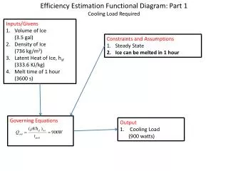
Efficiency Estimation Functional Diagram: Part 1 Cooling Load Required Inputs/Givens Volume of Ice (3.5 gal) Density of Ice (736 kg/m3) Latent Heat of Ice, hsf (333.6 KJ/kg) Melt time of 1 hour (3600 s) Constraints and Assumptions Steady State Ice can be melted in 1 hour Governing Equations Output Cooling Load (900 watts)
Efficiency Estimation Functional Diagram: Part 2 Fan/Pump sizing Constraints and Assumptions Ideal gas Incompressible flow Constant Pressure (Cp) Uniform Flow Steady State Ambient air Temp of 22 C and output temp of 13 C Coolant temp of 0 C from ice box Ice can be melted in 1 hour Inputs/Givens Heat Flux (900W) Fluid properties of air and water Governing Equations Output Air Flow Rate (0.12 m3/s) Coolant Flow Rate (1 GPM -> at least 0.5)
Efficiency Estimation Functional Diagram: Part 3 COP calculation Input data Cooling Load (900 watts) Coolant Flow rate (1 GPM -> at least 0.5) Governing Equations Output COP = 10 Constants and Knowns Density of Water (1000 kg/m3) Constraints and Assumptions No pumping losses 65% pump efficiency (low) Fan at 100%power Steady State 2x calculated pump power to accommodate losses z (H) of coolant in pumping loop equal to 1m (would be less in actual unit)
Final Efficiency Functional Diagram (Final Testing) Measured data Tof water in and out of radiator Win from “plug power meter” Coolant Flow Rate Governing Equations Output Final/Overall COP of unit Constants and givens Area, A, of air flow Fluid properties of air (density, Cp) • Constraints and Assumptions- Ideal gas • Incompressible flow • Constant Pressure (Cp) • Uniform Flow
Final Efficiency Functional Diagram (Final Testing) Measured data Tof water in and out of radiator Win from “plug power meter” Coolant Flow Rate Governing Equations Output Final/Overall COP of unit Constants and givens Area, A, of air flow Fluid properties of air (density, Cp) • Constraints and Assumptions- Ideal gas • Incompressible flow • Constant Pressure (Cp) • Uniform Flow