Recognition Using SIFT Features
Recognition Using SIFT Features. CS491Y/691Y Topics in Computer Vision Dr. George Bebis. Object Recognition. Model-based Object Recognition Generic Object Recognition. Model-Based Object Recognition. Recognition relies upon the existence of a set of predefined objects.


Recognition Using SIFT Features
E N D
Presentation Transcript
Recognition Using SIFT Features CS491Y/691Y Topics in Computer Vision Dr. George Bebis
Object Recognition • Model-based Object Recognition • Generic Object Recognition
Model-Based Object Recognition • Recognition relies upon the existence of a set of predefined objects.
Feature-based Recognition • Identify a group of features from an unknown scene which approximately match a group of features from a model object (i.e., correspondences). (2) Recover the geometric transformation that the model object has undergone and look for additional matches. scene model
2D Transformation Spaces • Rigid transformations (3 parameters) • Similarity transformations (4 parameters) • Affine transformations (6 parameters)
Matching – Main Steps • Hypothesis generation: the identities of one or more models are hypothesized. • Hypothesis verification: tests are performed to check if a given hypothesis is correct or not. Recognition
Hypothesis Verification - Example two hypotheses: Features might correspond to: (1) curvature extrema or zero-crossings along the boundary of an object . (2) interest points.
Object Recognition using SIFT features Match individual SIFT features from an image to a database of SIFT features from known objects (i.e., find nearest neighbors). 2. Find clusters of SIFT features belonging to a single object (hypothesis generation).
Object Recognition using SIFT features 3. Estimate object pose (i.e., recover the transformation that the model has undergone) using at least three matches. 4. Verify that additional features agree on object pose (hypothesis verification).
Nearest neighbor search • Linear search: too slow for large database • kD trees: become slow when k > 10
Nearest neighbor search (cont’d) • Approximate nearest neighbor search: • Best-bin-first [Beis et al. 97] (modification to kD-tree algorithm) • Examine only the N closest bins of the kD-tree • Use a heap to identify bins in order by their distance from query. • Can give speedup by factor of 1000 while finding nearest neighbor (of interest) 95% of the time. FLANN - Fast Library for Approximate Nearest Neighbors Marius Muja and David G. Lowe, "Fast Approximate Nearest Neighbors with Automatic Algorithm Configuration", International Conference on Computer Vision Theory and Applications, 2009
Estimate object pose • Now, given feature matches… • Find clusters of features corresponding to a single object. • Solve for transformation (e.g., affine transformation). scene model
Estimate object pose (cont’d) • Need to consider clusters of size >=3 • How do we find three “good” (i.e., true) matches?
Estimate object pose (cont’d) Pose clustering Each SIFT feature is associated with four parameters: For every match (mi, sj), estimate a similarity transformation between mi and sj (2D location, scale, orientation) (tx,ty,s,θ) vote
Estimate object pose (cont’d) • Transformation space is 4D: (tx, ty, s, θ) votes (tx,ty,s,θ) …. (t’x,t’y,s’,θ’)
Estimate object pose (cont’d) • Partial voting: vote for neighboring bins and use large bin size to better tolerate errors. • Transformations that accumulate at least three votes are selected (hypothesis generation). • Using model-scene matches, compute object pose (i.e., affine transformation) and apply verification.
Verification • Back-project model (i.e., interest points) on the scene and look for additional matches. • Discard outliers (i.e., incorrect matches) by imposing stricter matching constraints (e.g., half error). • Find additional matches and refine the transformation computed (i.e., iterative affine refinements). • Repeat until no additional matches can be found.
Verification (cont’d) • Additional verification: evaluate probability that match is correct. • Use Bayesian (probabilistic) model, to estimate the probability that a model is present based on the matching features. • Bayesian model takes into account: • Object size in image • Textured regions • Model feature count in database • Accuracy of fit Lowe, D.G. 2001. Local feature view clustering for 3D object recognition.IEEE Conference on Computer Vision and Pattern Recognition, Kauai, Hawaii, pp. 682–688.
Planar recognition Models
Planar recognition (cont’d) Test image • Reliably recognized at a rotation of 60° away from the camera. • Affine fit approximates perspective projection. • Only 3 points are needed for recognition.
3D object recognition Models
3D object recognition Test images • Only 3 keys are needed for recognition; extra keys provide robustness. • Affine model is no longer as accurate.
Origin 1: Texture recognition Texture is characterized by the repetition of basic elements or textons. Many times, it is the identity of the textons, not their spatial arrangement, that matters.
Origin 2: Document retrieval • Orderless document representation: • frequencies of words from a dictionarySalton & McGill (1983)
BoF for object categorization Need a “visual” dictionary! G. Cruska et al., "Visual Categorization with Bags of Keypoints", European Conference on Computer Vision, Czech Republic, 2004
BoF: main steps Characterize objects in terms of parts or local features
BoF: main steps Step 1: Feature extraction (e.g., SIFT features) …
BoF: main steps (cont’d) Step 2: Learn “visual” vocabulary … Feature extraction & clustering “visual” vocabulary
BoF: main steps (cont’d) … Clustering
BoF: main steps (cont’d) “Visual” vocabulary: cluster centers … Clustering
Example: K-means clustering Want to minimize sum of squared Euclidean distances between points xiand their nearest cluster centers mk
Example: K-means clustering Algorithm: Randomly initialize K cluster centers Iterate until convergence: Assign each data point to the nearest center. Re-compute each cluster center as the mean of all points assigned to it.
More powerful clustering algorithms Affinity propagation http://www.psi.toronto.edu/index.php?q=affinity%20propagation Autoclass http://ti.arc.nasa.gov/tech/rse/synthesis-projects-applications/autoclass/autoclass-c/
BoF: main steps (cont’d) Step 3: Quantize features using “visual” vocabulary (i.e., represent each feature by the closest cluster center). …
BoF: main steps (cont’d) Step 4: Represent images by frequencies of “visual words” (i.e., bags of features)
BoF Object Categorization How do we use BoF for object categorization?
BoF Object Categorization (cont’d) (1) Use a Nearest Neighbor (NN) Classifier
BoF Object Categorization (cont’d) Functions for comparing histograms
BoF Object Categorization (cont’d) (2) Use a K-Nearest Neighbor (KNN) Classifier Find the k closest points from training data. Labels of the k points “vote” to classify. Works well provided there is lots of data and the distance function is good.
BoF Object Categorization (cont’d) (3) Naïve Bayes classifier
BoF Object Categorization (cont’d) (3) Naïve Bayes classifier
BoF Object Categorization (cont’d) (3) Naïve Bayes classifier
BoF Object Categorization (cont’d) (3) Naïve Bayes classifier or
BoF Object Categorization (cont’d) (4) Use an SVM classifier SVM SVM SVM
Example Caltech6 dataset