Download
1 / 22
220 likes | 240 Views
Learn about particle filtering, a nonlinear method using sequential Monte Carlo techniques for signal prediction and filtering. Discover its application in speech recognition and various industries. Follow step-by-step procedures and practical examples.

E N D
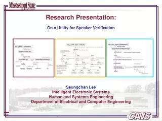
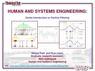
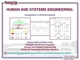
HUMAN AND SYSTEMS ENGINEERING: Introduction to Particle Filtering Sanjay Patil and Ryan Irwin Intelligent Electronics Systems Human and Systems Engineering Center for Advanced Vehicular Systems URL: www.cavs.msstate.edu/hse/ies/publications/seminars/msstate/2005/particle_filtering/
Abstract • The conventional techniques in speech recognition applications • model speech as Gaussian mixtures • lacks robustness to noise and mismatched channel • Nonlinear techniques • model speech as a time-varying and non-stationary signal • Particle filtering • a nonlinear method • based on sequential Monte Carlo techniques • a technique that can be used for prediction or filtering of signal • works by approximating the target probability distribution (e.g. amplitude of speech signal) • possible to increase the number of Gaussian mixtures to improve the prediction or filtering of signal.
200 samples 5000 samples 500 samples • Drawing samples to represent a probability distribution function • Particles and their weights • consider a pdf p(x) (blue line) • generate random samples (red lines) which can represent this pdf (N = # of samples) • Conclusion • approximation depends on • number (N) of samples • amplitude (x) of a sample (i) is its weight. each sample is called as ‘Particle’
Particle filtering algorithm Problem Statement – find what x is at a given time instant Observations: known can be measured (y1, y2, y3, y4 y5, y6, y7, … yk-2, yk-1, yk, ...) States: unknown (hence need to calculated) (x0, x1, x2, x3, x4 x5, x6, x7, … xk-2, xk-1, xk, … ) subscripts indicate time index.
Particle filtering algorithm continued General two-stage framework (Prediction-Update stages) • Assume that pdf p(xk-1 | y1:k-1) is available at time k -1. • Prediction stage: • This is a priori of the state at time k ( without the information on measurement). Thus, it is the probability of the state given only the previous measurements • Update stage: • This is posterior pdf from predicted prior pdf and newly available measurement.
Particle filtering algorithm step-by-step (1) Initial set-up: No observations available Known parameters – x0, p(x0), p(xk|xk-1), p(yk|xk), noise statistics Draw samples to represent x0 by its distribution p(x0) time Measurements / Observations States (unknown / hidden) cannot be measured N = 5 (1.00, -1.176, 0.427, 0.906, 1.072)
Particle filtering algorithm step-by-step (2) Known parameters – x0, p(x0), p(xk|xk-1), p(yk|xk), noise statistics Still no observations or measurements are available. Predict x1 using equation time Measurements / Observations States (unknown / hidden) cannot be measured (0.5370, -0.9480, 0.63080, 1.51697, 0.39145 )
Particle filtering algorithm step-by-step (3) Known parameters – x0, p(x0), p(xk|xk-1), p(yk|xk), noise statistics First observation / measurement is available. Update x1 using equation time Measurements / Observations 0.42 States (unknown / hidden) cannot be measured (0.5370, 0.63080, 0.630, 0.630, 1.0 ) 0.685
Particle filtering algorithm step-by-step (4) Known parameters – x0, p(x0), p(xk|xk-1), p(yk|xk), noise statistics Second observation / measurement is NOT available. Predict x2 using equation time Measurements / Observations States (unknown / hidden) cannot be measured (-1.651, 0.831, 1.888, 1.459, 2.540)
Particle filtering algorithm step-by-step (5) Known parameters – x0, p(x0), p(xk|xk-1), p(yk|xk), noise statistics Second observation / measurement is available. update x2 using equation time -0.01 Measurements / Observations States (unknown / hidden) cannot be measured (-1.651, -1.651, 0.831, 0.831, 1.0 ) -0.12
time Measurements / Observations States (unknown / hidden) cannot be measured • Particle filtering algorithm step-by-step (6) Known parameters – x0, p(x0), p(xk|xk-1), p(yk|xk), noise statistics kth observation / measurement is available. Predict and Update xk using equation
Particle filtering - visualization • Drawing samples • Predicting next state • Updating this state • What is THIS STEP??? • Resampling….
Applications • Most of the applications involve tracking • Visual Tracking – e.g. human motion (body parts) • Prediction of (financial) time series – e.g. mapping gold price, stocks • Quality control in semiconductor industry • Military applications • Target recognition from single or multiple images • Guidance of missiles • For IES NSF funded project, particle filtering has been used for: • Time series estimation for speech signal (Java demo) • Speaker Verification (details on next slide)
Speaker Verification • Time series estimation of speech signal • Speaker Verification: • Hypothesis: particle filters approximate the probability distribution of a signal. If large number of particles are used, it approximates the pdf better. Only needed is the initial guess of the distribution. • ! How are we going to achieve this..
Pattern Recognition Applet • Java applet that gives a visual of algorithms implemented at IES • Classification of Signals • PCA - Principle Component Analysis • LDA - Linear Discrimination Analysis • SVM - Support Vector Machines • RVM - Relevance Vector Machines • Tracking of Signals • LP - Linear Prediction • KF - Kalman Filtering • PF – Particle Filtering URL: http://www.cavs.msstate.edu/hse/ies/projects/speech/software/demonstrations/applets/util/pattern_recognition/current/index.html
Classification – Best Case • Data sets need to be differentiated • Classifying distinguishes between sets of data without the samples • Algorithms separate data sets with a line of discrimination • To have zero error the line of discrimination should completely separate the classes • These patterns are easy to classify
Classification – Worst Case • Toroidals are not classified easily with a straight line • Error should be around 50% because half of each class is separated • A proper line of discrimination of a toroidal would be a circle enclosing only the inside set • The toroidal is not common in speech patterns
Classification – Realistic Case • A more realistic case of two mixed distributions using RVM • This algorithm gives a more complex line of discrimination • More involved computation for RVM yields better results than LDA and PCA • Again, LDA, PCA, SVM, and RVM are pattern classification algorithms • More information given online in tutorials about algorithms
Signal Tracking – Kalman Filter • The input signals are now time based with the x-axis representing time • Signal tracking algorithms interpolate data • Interpolation ensures that the input samples are at regular intervals • Sampling is always done on regular intervals • Kalman filter is shown here
Signal Tracking – Particle Filter • Algorithm has realistic noise • Gaussian noise is actually generated at each step • Noise variances and number of particles can be customized • Algorithm runs as previously described • State prediction stage • State update stage • Average of the black particles is where the overall state is predicted
Summary • Particle filtering promises to be one of the nonlinear techniques. • More points to follow
References • S. Haykin and E. Moulines, "From Kalman to Particle Filters," IEEE International Conference on Acoustics, Speech, and Signal Processing, Philadelphia, Pennsylvania, USA, March 2005. • M.W. Andrews, "Learning And Inference In Nonlinear State-Space Models," Gatsby Unit for Computational Neuroscience, University College, London, U.K., December 2004. • P.M. Djuric, J.H. Kotecha, J. Zhang, Y. Huang, T. Ghirmai, M. Bugallo, and J. Miguez, "Particle Filtering," IEEE Magazine on Signal Processing, vol 20, no 5, pp. 19-38, September 2003. • N. Arulampalam, S. Maskell, N. Gordan, and T. Clapp, "Tutorial On Particle Filters For Online Nonlinear/ Non-Gaussian Bayesian Tracking," IEEE Transactions on Signal Processing, vol. 50, no. 2, pp. 174-188, February 2002. • R. van der Merve, N. de Freitas, A. Doucet, and E. Wan, "The Unscented Particle Filter," Technical Report CUED/F-INFENG/TR 380, Cambridge University Engineering Department, Cambridge University, U.K., August 2000. • S. Gannot, and M. Moonen, "On The Application Of The Unscented Kalman Filter To Speech Processing," International Workshop on Acoustic Echo and Noise, Kyoto, Japan, pp 27-30, September 2003. • J.P. Norton, and G.V. Veres, "Improvement Of The Particle Filter By Better Choice Of The Predicted Sample Set," 15th IFAC Triennial World Congress, Barcelona, Spain, July 2002. • J. Vermaak, C. Andrieu, A. Doucet, and S.J. Godsill, "Particle Methods For Bayesian Modeling And Enhancement Of Speech Signals," IEEE Transaction on Speech and Audio Processing, vol 10, no. 3, pp 173-185, March 2002.