Active Contours without Edges
Active Contours without Edges. Tony Chan Luminita Vese. Peter Horvath – University of Szeged 29/09/2006 . Introduction. Variational approach The main problem is to minimise an integral functional (e.g.): In the case f: , f’=0 gives the extremum(s)


Active Contours without Edges
E N D
Presentation Transcript
Active Contours without Edges Tony Chan Luminita Vese Peter Horvath – University of Szeged 29/09/2006
Introduction • Variational approach • The main problem is to minimise an integral functional (e.g.): • In the case f:, f’=0 gives the extremum(s) • In the case of functionals similary F’=0, where F’=(F/u) is the first variation. • Most of the cases the solution is analyticly hard, in these cases we use gradient descent to optimise.
Introduction • Active Contour (Snake Model) • Kass, Witkin and Terzopoulos [Kas88] • - tension • - rigidity • Eext – external energy • Problem is: infxE + Fast evaluation - But difficult to handle topological changes
Introduction • A typical external energy coming from the image: • Positive on homogeneous regions • Near zero on the sharp edges
Intoduction • Level Set methods • S.Osher and J. Sethian [Set89] • Embed the contour into a higher dimensional space +Automatically handles the topological changes - Slower evaluation • (., t) level set function • Implicit contour (=0) • The contour is evolved implicitly by moving the surface
Introduction • The curve is moving with an F speed: • The geometric active contour, based on a mean curvature (length) motion:
Chan and Vese model position Energy functionals for image segmentation • Important to distinguish the model and the representation • Model: describing problems from the real world with equations • Representation: type of the description • Optimization: solving the equations Chan and Vese model Representation/optimization Contour basedgradient descent Level set basedgradient descent
Chan and Vese model • The model is based on trying to separate the image into regions based on intensities • The minimization problem:
Chan and Vese model • c1 and c2 are the average intensity levels inside and outside of the contour • Experiments:
Relation with the Mumford-Shah functional • The Chan and Vese model is a special case of the Mumford Shah model (minimal partition problem) • =0 and 1=2= • u=average(u0 in/out) • C is the CV active contour • “Cartoon” model
Level set formulation • Considering the disadvantages of the active contour representation the model is solved using level set formulation • level set form -> no explicit contour
Replacing C with Φ • Introducing the Heaviside (sign) and Dirac (PSF) functions
Replacing C with Φ • The intensity terms
Average intensities • We can calculate the average intensities using the step function
Level set formulation of the model Combining the above presented energy terms we can write the Chan and Vese functional as a function of Φ. Minimization F wrt. Φ -> gradient descent The corresponding Euler-Lagrange equation:
The algorithm • Initialization n=0 • repeat • n++ • Computing c1 and c2 • Evolving the level-set function • until the solution is stationary, or n>nmax
Initialization • We set the values of the level set function • outside = -1 • inside = 1 • Any shape can be the initialization shape init() for all (x, y) in Phi if (x, y) is inside Phi(x, y)=1; else Phi(x, y)=-1; fi; end for
Computing c1 and c2 • The mean intensity of the image pixels inside and outside colors() out = find(Phi < 0); in = find(Phi > 0); c1 = sum(Img(in)) / size(in); c2 = sum(Img(out)) / size(out);
Finite differences for all (x, y) fx(x, y) = (Phi(x+1, y)-Phi(x-1, y))/(2*delta_s); fy(x, y) =… fxx(x, y) =… fyy(x, y) =… fxy(x, y) =… delta_s recommended between 0.1 and 1.0
Curvature grad = (fx.^2.+fy.^2); curvature = (fx.^2.*fyy + fy.^2.*fxx - 2.*fx.*fy.*fxy) ./ (grad.^1.5); Be careful! Grad can be 0!
Force gradient_m = (fx.^2.+fy.^2).^0.5; force = mu * curvature .* gradient_m - nu – lambda1 * (image - c1).^2 + lambda2 * (image - c2).^2; We should normalize the force. abs(force) <= 1! Main step: Phi=Phi+deltaT*force; deltaT is recommended between 0.01 and 0.9. Be careful deltaT<1!
Narrow band It is useful to compute the level set function not on the whole image domain but in a narrow band near to the contour. Abs()<d Decreasing the computational complexity.
Narrow band • Initialization n=0 • repeat • n++ • Determination of the narrow band • Computing c1 and c2 • Evolving the level-set function on the narrow band • Re-initialization • until the solution is stationary, or n>nmax
Re-initialization • Optional step H is a normalizing term recommended between 0.1 and 2. deltaT time step see above!
Stop criteria • Stop the iterations if: • The maximum iteration number were reached • Stationary solution: • The energy is not changing • The contour is not moving • …
Demonstration of the program • Thanks for your attention
MATLAB tutorial • Imread, imwrite • .*, .^, ./ • Find • Size, length, max, min, mod, sum, zeros, ones • A(x:y, z:v) • Visualization: figure, plot, surf, imagesc