Working With Basic Aggregate Demand/Supply Model
430 likes | 446 Views
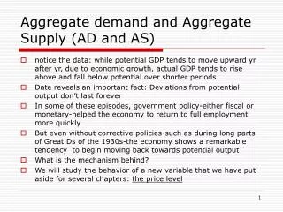
Learn about the Aggregate Demand curve, factors shifting AD, Short-Run Aggregate Supply, Long-Run Aggregate Supply, and how changes impact an economy.

Working With Basic Aggregate Demand/Supply Model
E N D
Presentation Transcript
Chapter 10 Working With Basic Aggregate Demand/Supply Model
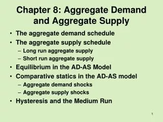
Aggregate Demand for Goods & Services • Aggregate demand curve:-- indicates the various quantities of domestically produced goods & services that purchasers are willing to buy at different price levels . • The AD curve slopes downward to the right, indicating an inverse relationship between the amount of goods & services demanded and the price level.
Price level A reduction in the price level will increase the quantity of goods &services demanded. P 1 P 2 AD Goods &Services(real GDP) Y Y 1 2 Aggregate Demand Curve
Why Does the Aggregate Demand Curve Slope Downward • The Wealth Effect:A lower price level will increase the purchasing power of the fixed quantity of money. • The Interest Rate Effect: A lower price level will make the nominal interest rate appear lower which will stimulate additional purchases during the current period. • The Foreign Purchases Effect:Other things constant, a lower price level will make domestically produced goods less expensive relative to foreign goods.
Factors that Shift Aggregate Demand • A decrease (increase) in Consumer Debt. • An increase in the optimism (pessimism) of businesses and consumers about future economic Expectations. • An increase (decrease) in Taxes. • An increase (decrease) in Real Wealth.
Price level AD 1 Goods &Services(real GDP) AD 0 AD 2 Shifts in Aggregate Demand
Aggregate Supply of Goods & Services • When considering the Aggregate Supply curve, it is important to distinguish between the short-run and the long-run. • Short-run:-- time period during which some prices, particularly those in resource markets, are set by prior contracts and agreements. Therefore, in the short-run, households and businesses are unable to adjust these prices when unexpected changes occur, including unexpected changes in the price level. • Long-run:-- a time period of sufficient duration that people have the opportunity to modify their behavior in response to economic changes.
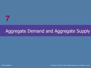
Short-Run Aggregate Supply (SRAS) • SRAS indicates the various quantities of goods & services that domestic firms will supply in response to changing demand conditions that alter the level of prices in the goods & services market. • SRAS curve slopes upward to the right. • The upward slope reflects the fact that in the short run an unanticipated increase in the price level will improve the profitability of firms and they will respond with an expansion in output.
Price level SRAS (P100) P 105 An increase in the price level will increase the quantity supplied in the short run. P 100 P 95 Goods &Services(real GDP) Y Y Y 1 2 3 Short-Run Aggregate Supply Curve
Shifts in Aggregate Supply • Factors that change SRAS: • A decrease (increase) in resource prices — that is, production costs such as wages, rent, and interest. • A reduction (increase) in the expected rate of inflation. • Favorable (unfavorable) supply shocks, such as good (bad) weather or a reduction (increase) in the world price of a key imported resource.
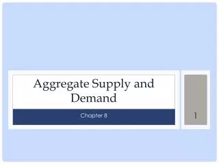
Long-Run Aggregate Supply (LRAS) • LRAS indicates the relationship between the price level and quantity of output after decision makers have had sufficient time to adjust their prior commitments where possible. • LRAS curve is vertical. • LRAS is related to the economy's production possibilities frontier. A higher price level does not loosen the constraints imposed by the economy's resource base, level of technology, and the efficiency of its institutional arrangements.
Price level LRAS Change in price level does not affect quantity supplied in the long run. Potential GDP Goods &Services(real GDP) Y (full employment rate of output) F Long-Run Aggregate Supply Curve
Anticipated and Unanticipated Changes • Anticipated changes are foreseen by economic participants. • Decision makers have time to adjust to them before they occur. • Unanticipated changes catch people by surprise.
Unanticipated Changes in Aggregate Demand • Impact of unanticipated reductions in AD: • Weak demand and lower prices in the goods & services market will reduce profit margins. Many firms will incur losses. • Firms will reduce output, the rate of unemployment will rise above the natural rate, and output will temporarily fall short of the economy's long-run potential. • With time, long-term contracts will be modified. • Eventually, lower resource prices and a lower real interest rate will direct the economy back to long-run equilibrium, but this may be a lengthy and painful process.
Price level LRAS SRAS1 Short-run effects of an unanticipated reduction in AD P P 95 100 AD2 AD1 Goods &Services(real GDP) Y Y F 2 Unanticipated Reduction in Aggregate Demand • The short-run impact of an unanticipated reduction in AD (shift from AD1 to AD2) will be a decline in output (decreases to Y2), and a lower price level (P95). • Temporarily, profit margins decline, output falls, and unemployment rises below its natural rate.
LRAS SRAS2 Long-run effects of an unanticipated reduction in AD P P P 95 90 100 AD2 Y Y Y F F 2 Unanticipated Reduction in Aggregate Demand Price level SRAS1 AD1 Goods &Services(real GDP) • In the long-run, weak demand and excess supply in the resource market will lead to lower wage rates and resource prices resulting in an expansion in short-run aggregate supply to SRAS2. • In the long-run, a new equilibrium at a lower price level (P90) and an output consistent with the economy’s sustainable potential will result. • This method of restoring equilibrium may be both long and painful.
Unanticipated Changes in Aggregate Demand • Impact of unanticipated increases in AD: • Initially, the strong demand and higher price level in the goods & services market will temporarily improve profit margins. • Output will increase, the rate of unemployment will drop below the natural rate, and output will temporarily exceed the economy's long-run potential. • With time, however, contracts will be modified and resource prices will rise and return to their competitive relation with product prices. • Once this happens, output will recede to the economy's long-run potential.
Price level LRAS SRAS1 Short-run effects of an unanticipated increase in AD P P 100 105 AD2 AD1 Goods &Services(real GDP) Y Y F 2 Unanticipated Increase in Aggregate Demand • In response to an unanticipated increase in AD for goods & services (shift from AD1 to AD2), prices will rise to P105 and output will temporarily exceed full-employment capacity (increases to Y2).
LRAS SRAS2 Long-run effects of an unanticipated increase in AD P P P 110 100 105 Y Y Y 2 F F Unanticipated Increase in Aggregate Demand Price level SRAS1 AD2 AD1 Goods &Services(real GDP) • With the passage of time, prices in resource markets, including the labor market, will rise due to the strong demand. As a result, higher costs reduce aggregate supply to SRAS2. • In the long-run, a new equilibrium at a higher price level (P110) and an output consistent with the economy’s sustainable potential will occur. • Thus, the increase in demand will expand output only temporarily.
Shifts in Long Run Aggregate Supply • Factors that change LRAS: • An increase (decrease) in the supply of resources. • An improvement (deterioration) in technology and productivity. • Institutional changes that increase (reduce) the efficiency of resource use such as trade agreements.
Impact of Changes in Aggregate Supply • Economic growth and anticipated shifts in long-run aggregate supply. • Increases in LRAS will make it possible to produce and sustain a larger rate of output. • Both LRAS and SRAS will shift to the right and output will increase. • These changes generally take place slowly and therefore they need not disrupt long-run equilibrium.
Price level Price level LRAS1 LRAS2 SRAS1 SRAS2 Y Y Goods &Services(real GDP) Goods &Services(real GDP) F,1 F,2 Shifts in Aggregate Supply • Such factors as an increase in the stock of capital or an improvement in technology will expand the economy’s potential output and shift the LRAS to the right (note that SRAS will also shift to the right). • Such factors as a reduction in resource prices, favorable weather, or a temporary decrease in the world price of an important imported resource would shift SRAS to the right (note that LRAS will remain constant).
LRAS1 LRAS2 Price level SRAS1 SRAS2 P P 1 2 AD Goods &Services(real GDP) Y Y Y Y F2 F2 F1 F Growth in Aggregate Supply • Here we illustrate the impact of economic growth due to capital formation or a technological advancement, for example. • Both LRAS and SRASincrease (to LRAS2 and SRAS2); the full employment output of the economy expands from YF1 to YF2. • A sustainable, higher level of real output and real income is the result. If the money supply is held constant, a new long-run equilibrium will emerge at a larger output rate (YF2) and lower price level (P2).
The Business Cycle-- Revisited • Recessions occur because prices in the goods & services market are low relative to the costs of production and resource prices. • The two causes of recessions: • unanticipated reductions in aggregate demand, and, • unfavorable supply shocks. • An unsustainable economic boom occurs when prices in the goods & services market are high relative to costs and resource prices. • The two causes of booms are: • unanticipated increases in aggregate demand, and, • favorable supply shocks.
Expansion Expansion Real GDP(billions of 1987 $) 6,000 1990 Recession 4,000 RealGDP 1982 Recession 1980 Recession 1974–75 2,000 Recession 1970 Recession 1960 Recession 0 1960 1965 1970 1975 1980 1985 1990 1995 2000 Actual rate of unemployment Percentage of the Labor Force Unemployed Natural rate of unemployment(estimated range) 10 8 6 4 2 0 2000 1960 1965 1970 1975 1980 1985 1990 1995 Source: Derived from computerized data supplied by FAME Economics. Expansions, Recessions, and the Rate of Unemployment • Here we illustrate the periods of expansion and contraction (recession) since 1960. • Note how the reductions in real GDP (shaded periods) in the top graph are associated with increases in the rate of unemployment well above the natural rate (bottom graph). • The AD/AS model indicates that recessions are caused by unanticipated reductions in AD that are likely to accompany abrupt reductions in the inflation rate and/or adverse supply shocks that might occur, for example, when there is a large increase in the price of a key imported resource, such as crude oil.
Does the Market Have a Self-Corrective Mechanism That Will Keep it on Track?
Does the Market Have a Self-Corrective Mechanism That Will Keep it on Track? • There are three reasons to believe that it does: • Consumption demand is relatively stable over the business cycle. • Changes in real interest rates will help to stabilize aggregate demand and redirect economic fluctuations. • Interest rates will tend to fall during a recession and rise during and economic boom. • Changes in real resource prices will redirect economic fluctuations. • Real resource price will tend to fall during a recession and rise during an economic expansion.
LRAS Price level P P r r Goods &Services(real GDP) Unemployment greaterthan Natural Rate Unemployment lessthan Natural Rate Y F Changes in Real Interest Rates and Resource Prices Over the Business Cycle Real interest rates rise (because of strongdemand for investment) Real interest rates fall (because of weak demand for investment) r r Real resource prices fall (because of weak demand and high unemployment) Real resource prices rise (because of strong demand and low unemployment) • When aggregate output is less than the economy’s full employment potential (YF), weak demand for investment leads to lower real interest rates, while slack employment in resource markets will place downward pressure on wages and other resource prices (Pr). • Conversely, when output exceeds YF, strong demand for capital goods and tight labor market conditions will result in rising real interest rates and resource prices (Pr).
Price level LRAS SRAS1 SRAS2 Lower resource prices increaseSRAS Lower real interest rates increaseAD P P P 100 95 105 In the short-run, outputmay exceed or fall short of the economy’s full-employment capacity (YF). Goods &Services(real GDP) AD1 AD2 Y Y Y Y F 1 F F The Economy’s Self Corrective Mechanism • If output is temporarily less than capacity, lower interest rates (reflecting the weak demand for investment funds) will stimulate aggregate demand (shifting AD from AD1 to AD2). • In addition, lower resource prices will reduce production prices (because of weak demand and abnormally high unemployment) and thereby stimulate SRAS (shifting SRAS to SRAS2). • This output will move the economy toward full-employment capacity. However, this self-correction process may take some time.
Price level LRAS SRAS2 SRAS1 Higher resource prices reduceSRAS Higher real interest rates reduceAD P P P 105 95 100 In the short-run, outputmay exceed or fall short of the economy’s full-employment capacity (YF). AD1 AD2 Goods &Services(real GDP) Y Y Y Y F 1 F F The Economy’s Self Corrective Mechanism • If output is temporarily greater than the economy’s potential, higher real interest rates and resource prices will lead to a lower but sustainable rate of output. • Higher interest rates will reduce AD (from AD1 to AD2). • At the same time, higher resource prices will increase production costs and therefore reduce SRAS (from SRAS1 to SRAS2). • These forces direct output toward full-employment potential (YF).
The Great Debate:-- How rapidly does the self-corrective mechanism work?
The Great Debate:-- How rapidly does the self-corrective mechanism work? • Many economists believe that the self-corrective mechanism works slowly. • If this is the case, then market economies will still experience prolonged periods of abnormally high unemployment and below-capacity output. • Others believe that the self-corrective mechanism works fairly rapidly if it is not disrupted by perverse monetary and fiscal policy. • This is an important and continuing debate that we will return to and analyze in more detail as we proceed.