Download
1 / 37
370 likes | 504 Views
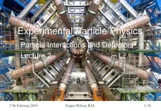
Physics 214 UCSD Physics 225a UCSB Experimental Particle Physics. Lecture 2 Fast forward through HEP Detectors. Quark Model. At this point it should be obvious that you can construct a large variety of baryons and mesons simply by angular momentum addition. All of them will be color neutral.

E N D
Physics 214 UCSDPhysics 225a UCSBExperimental Particle Physics Lecture 2 Fast forward through HEP Detectors
Quark Model • At this point it should be obvious that you can construct a large variety of baryons and mesons simply by angular momentum addition. • All of them will be color neutral. • Lowest lying states for a given flavor composition are stable with regard to strong interaction but not weak interaction. • Excited states can be made by adding orbital angular momentum of the quarks with respect to each other. • Excited states are not stable with respect to strong interactions.
However, nature’s more complicated still. The quarks from quantum fluctuations are called sea quarks. You can probe sea quarks and gluons inside hadrons by scattering electrons off hadrons at high momentum transfer.
Interactions mediated by vector bosons Tempting to think about the exchange as a quantum fluctuation.
Range of “force” as quantum fluctuation R 1/m Range of force is inverse proportional to mass of mediator.
Well, I’m cheating a little • We will see that this works because: • Cross section |A|2 • A is perturbative expansion in Feynman diagrams. • Diagrams include vertex factors and propagators. • Propagators are interpreted as “mediators” of the interaction. • If you wish, the mental picture works because perturbation theory works.
A bit more rigorous: Yukawa Static source of “charge” => Spherical potential. As solution to: Given that QM tells us:
Add to this Fermi’s Golden Rule: • Incoming plane wave => outgoing whatever • Rate of transition = 2 |Mif|2 (Ef) • With: Mif = f* U(r) i dVol • As the wave functions are plane waves, this is nothing more than the fourier transform of the potential, with k being the momentum transfer in the collission.
Things to remember: • Rate of transition |Amplitude|2 • Amplitude = vertex factors * propagator All of this is for single boson exchange, i.e. leading order process only!
Rules for Standard Model Interactions Note: The formalism is the same with new physics. All you do is add new particles and rules for the interactions.
Orders of magnitude of interactions: Can we understand these numbers? Note: 1 barn = 10-28 m2
1st order = coupling2 x propagator2 s EM ~104 EM & Strong mediated by massless particles … … but with different couplings. EM & weak have ~ same coupling … … but with different mass for propagator. Processes we listed have roughly k~1GeV Impressive how well these simple relative estimates work!
What about estimating the absolute scale? Assume pion-proton scattering is nothing more than Solid sphere’s hitting each other: ~ A ~ R2 ~ 3 (1fm)2 ~ 30mb Lifetime of strong decaying particle is defined by range based on exchange of lightest colorless hadron: ~ 1/m ~ 1/100MeV ~ 10-23 sec
Couplings depend on momentum transfer, Q Strong coupling is O(1) at the scale of hadron masses, thus confinement, but becomes O(0.1), and thus perturbative, at O(100GeV), i.e. asymptotic freedom. hep-ph/0012288v2
Coupling Unification ??? • The “Q” here is • actually k2/2, with • being a reference scale, e.g. MZ , at which the couplings are measured. Details of the running depends on gauge boson self-couplings, # of families, and # of Higgs doublets, and Particle content and Masses in the theory. hep-ph/0012288v2
Issues around unstable particles (1) • Assume we have a large number N of particles of a certain type, at t=t0. How many are left at t=t0+dt ? p(t)dt = prob. for decay during dt := k dt P(t) = prob. for survival at t Exponential decay law follows directly from assumption of constant rate of decay, i.e. transition rate that is independent of N(t=0).
Issues around unstable particles (2) • We refer to as the “lifetime” of the particle because <t>decay = • We refer to =1/ as the Total Width, or total decay rate. • In general, a particle may decay via more than one path, or into more than one distinct final state. E.g. Z->e+e- , +-, etc. We refer to the decay rate into a given final state as the partial with, i . • The total width is given by the sum of all partial widths. • We refer to the ratio of i / as the “branching ratio” into the final state i. • The sum of all branching ratios adds up to 1.
Issues around unstable particles (3) • What’s the mass of an unstable particle? E t ~ 1 In rest frame E=M, In general t ~ , => M ~ • If mass isn’t well defined, then what’s the probability distribution for finding a particle with a given mass? • We call this the “lineshape” of the particle. Normalization for stable particle. Normalization for unstable particle.
We can get to this normalization of we replace: E0 by E0 - i /2 . We then get the lineshape from fourier transformation: Identify E with M and you get the non-relativistic Breit-Wigner lineshape.
In real live, hadronic resonances are not this simple because … • Interference with higher resonances. • Total width depends on M. • Phase space affects lineshape • Finite size effects (Blatt-Weisskopf barrier penetration factor) I’ll show you examples for the first 3, and refer you to references for further reading: http://mit.fnal.gov/~fkw/teaching/references/1018.html This page has links to the original papers for the plots I am showing, as well as a memo on BW’s et al. by Alan Weinstein, Caltech.
Interference with higher resonances Data from tau decays to two pions at CLEO. Dotted line is without a rho’. Solid line with. The data clearly demands the rho’. (Feel free to look up rho and rho’ in the PDG)
Mass dependent width Data from tau decays to three pions at CLEO. The data requires that one allows for a K*K partial width once allowed kinematically. However, even without it, the total width increases significantly as a function of 3-pion invariant mass. (Feel free to look up the a1 in PDG)
Lineshape sculpting due to phase space constraints. Note: The f0 is actually wider on the high side than the low side because of the KK kinematic threshold!
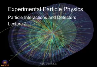
Switch gear now! Let’s talk about detectors for a bit. Let’s do this with Atlas and CMS in mind. Suggested References: Kleinknecht (on reserve) CMS physics TDR vol. 1 (on the web at: http://cmsdoc.cern.ch/cms/cpt/tdr/ )
What do we need to detect? • Momenta of all stable particles: • Charged: Pion, kaon, proton, electron, muon • Neutral: photon, K0s , neutron, K0L , neutrino • Particle identification for all of the above. • “Unstable” particles: • Pizero • b-quark, c-quark, tau • Gluon and light quarks • W,Z,Higgs • … anything new we might discover …
All modern collider detectors look alike beampipe tracker ECAL solenoid Increasing radius HCAL Muon chamber
Tracking • Zylindrical geometry of central tracking detector. • Charged particles leave energy in segmented detectors. • Determines position at N radial layers • Solenoidal field forces charged particles onto helical trajectory • Curvature measurement determines charged particle momentum. • Limits to precision are given by: • Precision of each position measurement • Number of measurements • B field and lever arm • Multiple scattering
Momentum Resolution Two contributions with different dependence on pT Device resolution Multiple cattering Will go through multiple scattering in more detail next week
ECAL • Detects electrons and photons via energy deposited by electromagnetic showers. • Electrons and photons are completely contained in the ECAL. • ECAL needs to have sufficient radiation length X0 to contain particles of the relevant energy scale. • Energy resolution 1/E We will talk more about this next week.
HCAL • Only stable hadrons and muons reach the HCAL. • Hadrons create hadronic showers via strong interactions, except that the length scale is determined by the nuclear absorption length , instead of the electromagnetic radiation length X0 for obvious reason. • Energy resolution 1/E
“Compensating” Calorimeter • Due to isospin, roughly half as many neutral pions are produced in hadronic shower than charged pions. • However, only charged pions “feed” the hadronic shower as pi0 immediately decay to di-photons, thus creating an electromagnetic component of the shower. • Resolution is best if the HCAL has similar energy response to the EM part of the shower as the hadronic part. One of the big differences between ATLAS and CMS is that ATLAS HCAL is compensating, while CMS has a much better ECAL but a much worse HCAL response to photons.
Muon Detectors • Muons are minimum ionizing particles, i.e. small energy release, in all detectors. • Thus the only particles that range through the HCAL. • Muon detectors generally are another set of tracking chambers, interspersed with steal or iron absorbers to stop any hadrons that might have “punched through” the HCAL.