Download
1 / 68
700 likes | 995 Views
Fundamentals of Linear Algebra, Part II. Class 2. 31 August 2009 Instructor: Bhiksha Raj. Administrivia. Registration: Anyone on waitlist still? We have a second TA Sohail Bahmani sbahmani@andrew.cmu.edu Homework: Slightly delayed Linear algebra Adding some fun new problems.

E N D
Fundamentals of Linear Algebra, Part II Class 2. 31 August 2009 Instructor: Bhiksha Raj 11-755/18-797
Administrivia • Registration: Anyone on waitlist still? • We have a second TA • Sohail Bahmani • sbahmani@andrew.cmu.edu • Homework: Slightly delayed • Linear algebra • Adding some fun new problems. • Use the discussion lists on blackboard.andrew.cmu.edu • Blackboard – if you are not registered on blackboard please register 11-755/18-797
Overview • Vectors and matrices • Basic vector/matrix operations • Vector products • Matrix products • Various matrix types • Matrix inversion • Matrix interpretation • Eigenanalysis • Singular value decomposition 11-755/18-797
The Identity Matrix • An identity matrix is a square matrix where • All diagonal elements are 1.0 • All off-diagonal elements are 0.0 • Multiplication by an identity matrix does not change vectors 11-755/18-797
Diagonal Matrix • All off-diagonal elements are zero • Diagonal elements are non-zero • Scales the axes • May flip axes 11-755/18-797
Diagonal matrix to transform images • How? 11-755/18-797
Stretching • Location-based representation • Scaling matrix – only scales the X axis • The Y axis and pixel value are scaled by identity • Not a good way of scaling. 11-755/18-797
Stretching • Better way D = 11-755/18-797
Modifying color • Scale only Green 11-755/18-797
Permutation Matrix • A permutation matrix simply rearranges the axes • The row entries are axis vectors in a different order • The result is a combination of rotations and reflections • The permutation matrix effectively permutes the arrangement of the elements in a vector (3,4,5) Z (old X) 5 3 Y Y (old Z) Z 4 5 X 3 X (old Y) 4 11-755/18-797
Permutation Matrix • Reflections and 90 degree rotations of images and objects 11-755/18-797
Permutation Matrix • Reflections and 90 degree rotations of images and objects • Object represented as a matrix of 3-Dimensional “position” vectors • Positions identify each point on the surface 11-755/18-797
Rotation Matrix • A rotation matrix rotates the vector by some angle q • Alternately viewed, it rotates the axes • The new axes are at an angle q to the old one (x’,y’) y’ (x,y) (x,y) y q Y Y X X x’ x 11-755/18-797
Rotating a picture • Note the representation: 3-row matrix • Rotation only applies on the “coordinate” rows • The value does not change • Why is pacman grainy? 11-755/18-797
3-D Rotation Xnew • 2 degrees of freedom • 2 separate angles • What will the rotation matrix be? Ynew Y a Znew Z q X 11-755/18-797
Projections • What would we see if the cone to the left were transparent if we looked at it along the normal to the plane • The plane goes through the origin • Answer: the figure to the right • How do we get this? Projection 11-755/18-797
Projections • Each pixel in the cone to the left is mapped onto to its “shadow” on the plane in the figure to the right • The location of the pixel’s “shadow” is obtained by multiplying the vector V representing the pixel’s location in the first figure by a matrix A • Shadow (V )= A V • The matrix A is a projection matrix 11-755/18-797
Projections 90degrees • Consider any plane specified by a set of vectors W1, W2.. • Or matrix [W1 W2 ..] • Any vector can be projected onto this plane by multiplying it with the projection matrix for the plane • The projection is the shadow W2 W1 projection 11-755/18-797
Projection Matrix 90degrees • Given a set of vectors W1, W2, which form a matrix W = [W1 W2.. ] • The projection matrix that transforms any vector X to its projection on the plane is • P = W (WTW)-1 WT • We will visit matrix inversion shortly • Magic – any set of vectors from the same plane that are expressed as a matrix will give you the same projection matrix • P = V (VTV)-1 VT W2 W1 projection 11-755/18-797
Projections • HOW? 11-755/18-797
Projections • Draw any two vectors W1 and W2 that lie on the plane • ANY two so long as they have different angles • Compose a matrix W = [W1 W2] • Compose the projection matrix P = W (WTW)-1 WT • Multiply every point on the cone by P to get its projection • View it • I’m missing a step here – what is it? 11-755/18-797
Projections • The projection actually projects it onto the plane, but you’re still seeing the plane in 3D • The result of the projection is a 3-D vector • P = W (WTW)-1 WT= 3x3, P*Vector = 3x1 • The image must be rotated till the plane is in the plane of the paper • The Z axis in this case will always be zero and can be ignored • How will you rotate it? (remember you know W1 and W2) 11-755/18-797
Projection matrix properties • The projection of any vector that is already on the plane is the vector itself • Px = x if x is on the plane • If the object is already on the plane, there is no further projection to be performed • The projection of a projection is the projection • P (Px) = Px • That is because Px is already on the plane • Projection matrices are idempotent • P2 = P • Follows from the above 11-755/18-797
Projections: A more physical meaning • Let W1, W2 .. Wk be “bases” • We want to explain our data in terms of these “bases” • We often cannot do so • But we can explain a significant portion of it • The portion of the data that can be expressed in terms of our vectors W1, W2, .. Wk, is the projection of the data on the W1 .. Wk (hyper) plane • In our previous example, the “data” were all the points on a cone • The interpretation for volumetric data is obvious 11-755/18-797
Projection : an example with sounds • The spectrogram (matrix) of a piece of music • How much of the above music was composed of the above notes • I.e. how much can it be explained by the notes 11-755/18-797
Projection: one note • The spectrogram (matrix) of a piece of music M = W = • M = spectrogram; W = note • P = W (WTW)-1 WT • Projected Spectrogram = P * M 11-755/18-797
Projection: one note – cleaned up • The spectrogram (matrix) of a piece of music M = W = • Floored all matrix values below a threshold to zero 11-755/18-797
Projection: multiple notes • The spectrogram (matrix) of a piece of music M = W = • P = W (WTW)-1 WT • Projected Spectrogram = P * M 11-755/18-797
Projection: multiple notes, cleaned up • The spectrogram (matrix) of a piece of music M = W = • P = W (WTW)-1 WT • Projected Spectrogram = P * M 11-755/18-797
Projection and Least Squares • Projection actually computes a least squared error estimate • For each vector V in the music spectrogram matrix • Approximation: Vapprox = a*note1 + b*note2 + c*note3.. • Error vector E = V – Vapprox • Squared error energy for V e(V) = norm(E)2 • Total error = sum_over_all_V { e(V) } = SV e(V) • Projection computes Vapprox for all vectors such that Total error is minimized • It does not give you “a”, “b”, “c”.. Though • That needs a different operation – the inverse / pseudo inverse note1 note2 note3 11-755/18-797
Orthogonal and Orthonormal matrices • Orthogonal Matrix : AAT = diagonal • Each row vector lies exactly along the normal to the plane specified by the rest of the vectors in the matrix • Orthonormal Matrix: AAT = ATA = I • In additional to be orthogonal, each vector has length exactly = 1.0 • Interesting observation: In a square matrix if the length of the row vectors is 1.0, the length of the column vectors is also 1.0 11-755/18-797
Orthogonal and Orthonormal Matrices • Orthonormal matrices will retain the relative angles between transformed vectors • Essentially, they are combinations of rotations, reflections and permutations • Rotation matrices and permutation matrices are all orthonormal matrices • The vectors in an orthonormal matrix are at 90degrees to one another. • Orthogonal matrices are like Orthonormal matrices with stretching • The product of a diagonal matrix and an orthonormal matrix 11-755/18-797
Matrix Rank and Rank-Deficient Matrices • Some matrices will eliminate one or more dimensions during transformation • These are rank deficient matrices • The rank of the matrix is the dimensionality of the trasnsformed version of a full-dimensional object P * Cone = 11-755/18-797
Matrix Rank and Rank-Deficient Matrices • Some matrices will eliminate one or more dimensions during transformation • These are rank deficient matrices • The rank of the matrix is the dimensionality of the transformed version of a full-dimensional object Rank = 2 Rank = 1 11-755/18-797
Projections are often examples of rank-deficient transforms M = W = • P = W (WTW)-1 WT ; Projected Spectrogram = P * M • The original spectrogram can never be recovered • P is rank deficient • P explains all vectors in the new spectrogram as a mixture of only the 4 vectors in W • There are only 4 independent bases • Rank of P is 4 11-755/18-797
Non-square Matrices • Non-square matrices add or subtract axes • More rows than columns add axes • But does not increase the dimensionality of the data • Fewer rows than columns reduce axes • May reduce dimensionality of the data X = 2D data P = transform PX = 3D, rank 2 11-755/18-797
Non-square Matrices • Non-square matrices add or subtract axes • More rows than columns add axes • But does not increase the dimensionality of the data • Fewer rows than columns reduce axes • May reduce dimensionality of the data X = 3D data, rank 3 P = transform PX = 2D, rank 2 11-755/18-797
The Rank of a Matrix • The matrix rank is the dimensionality of the transformation of a full-dimensioned object in the original space • The matrix can never increase dimensions • Cannot convert a circle to a sphere or a line to a circle • The rank of a matrix can never be greater than the lower of its two dimensions 11-755/18-797
The Rank of Matrix M = • Projected Spectrogram = P * M • Every vector in it is a combination of only 4 bases • The rank of the matrix is the smallest no. of bases required to describe the output • E.g. if note no. 4 in P could be expressed as a combination of notes 1,2 and 3, it provides no additional information • Eliminating note no. 4 would give us the same projection • The rank of P would be 3! 11-755/18-797
Matrix rank is unchanged by transposition • If an N-D object is compressed to a K-D object by a matrix, it will also be compressed to a K-D object by the transpose of the matrix 11-755/18-797
Matrix Determinant (r1+r2) (r2) • The determinant is the “volume” of a matrix • Actually the volume of a parallelepiped formed from its row vectors • Also the volume of the parallelepiped formed from its column vectors • Standard formula for determinant: in text book (r1) (r2) (r1) 11-755/18-797
Matrix Determinant: Another Perspective Volume = V1 Volume = V2 • The determinant is the ratio of N-volumes • If V1 is the volume of an N-dimensional object “O” in N-dimensional space • O is the complete set of points or vertices that specify the object • If V2 is the volume of the N-dimensional object specified by A*O, where A is a matrix that transforms the space • |A| = V2 / V1 11-755/18-797
Matrix Determinants • Matrix determinants are only defined for square matrices • They characterize volumes in linearly transformed space of the same dimensionality as the vectors • Rank deficient matrices have determinant 0 • Since they compress full-volumed N-D objects into zero-volume N-D objects • E.g. a 3-D sphere into a 2-D ellipse: The ellipse has 0 volume (although it does have area) • Conversely, all matrices of determinant 0 are rank deficient • Since they compress full-volumed N-D objects into zero-volume objects 11-755/18-797
Multiplication properties • Properties of vector/matrix products • Associative • Distributive • NOT commutative!!! • left multiplications ≠ right multiplications • Transposition 11-755/18-797
Determinant properties • Associative for square matrices • Scaling volume sequentially by several matrices is equal to scaling once by the product of the matrices • Volume of sum != sum of Volumes • The volume of the parallelepiped formed by row vectors of the sum of two matrices is not the sum of the volumes of the parallelepipeds formed by the original matrices • Commutative for square matrices!!! • The order in which you scale the volume of an object is irrelevant 11-755/18-797
Matrix Inversion • A matrix transforms an N-D object to a different N-D object • What transforms the new object back to the original? • The inverse transformation • The inverse transformation is called the matrix inverse 11-755/18-797
Matrix Inversion T T-1 • The product of a matrix and its inverse is the identity matrix • Transforming an object, and then inverse transforming it gives us back the original object T-1T = I 11-755/18-797
Inverting rank-deficient matrices • Rank deficient matrices “flatten” objects • In the process, multiple points in the original object get mapped to the same point in the transformed object • It is not possible to go “back” from the flattened object to the original object • Because of the many-to-one forward mapping • Rank deficient matrices have no inverse 11-755/18-797
Revisiting Projections and Least Squares • Projection computes a least squared error estimate • For each vector V in the music spectrogram matrix • Approximation: Vapprox = a*note1 + b*note2 + c*note3.. • Error vector E = V – Vapprox • Squared error energy for V e(V) = norm(E)2 • Total error = Total error + e(V) • Projection computes Vapprox for all vectors such that Total error is minimized • But WHAT ARE “a” “b” and “c”? note1 note2 note3 11-755/18-797
The Pseudo Inverse (PINV) • We are approximating spectral vectors V as the transformation of the vector [a b c]T • Note – we’re viewing the collection of bases in W as a transformation • The solution is obtained using the pseudo inverse • This give us a LEAST SQUARES solution • If W were square and invertible Pinv(W) = W-1, and V=Vapprox 11-755/18-797