Download
1 / 25
250 likes | 408 Views
Density Curves. Section 2.1. Strategy to explore data on a single variable. Plot the data (histogram or stemplot) CUSS Calculate numerical summary to describe center and spread Mean and standard deviation Five number summary. From Histogram to Density Curve.

E N D
Density Curves Section 2.1
Strategy to explore data on a single variable • Plot the data (histogram or stemplot) • CUSS • Calculate numerical summary to describe center and spread • Mean and standard deviation • Five number summary
From Histogram to Density Curve Sometimes the overall pattern of a histogram can be described by a smooth curve.
Density Curve • Density curve is a mathematical model for the distribution • Idealized description • Scale is adjusted so area under the curve is equal to 1
Density Curve • A density curve is a curve that • Is always on or above the horizontal axis • Has area exactly 1 underneath it Describes the overall pattern of a distribution The area under the curve and above any range of values is the proportion of observations that fall in that range.
Uniform distribution • If the total area under the curve is 1, what is the height of the square? • What percent of the observations lie above 0.8? • What percent of the observations lie below 0.6? • What percent of the observations lie between 0.25 and 0.40?
1 1 0.5 0 0 0.5 1 1.5 2 2 Area under the curve • Is this a density curve?
Mean and Median of Density Curve • Mean is the point at which the curve would balance if it were made of solid material. • Median is the equal-areas point, the point that divides the area under the curve in half. • Mean and median are the same for symmetric curve.
Normal Distribution • Symmetric • Single-peaked • Bell-shaped • Can be defined by mean, m, and standard deviation, s.
68-95-99.7 Rule 68% of the observations fall within 1 standard deviation. 95% of the observations fall within 2 standard deviations. 99.7% of the observations fall within 3 standard deviations.
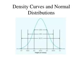
Example 2.3Young Women’s Heights • The distribution of heights of young women aged 18 to 24 is approximately normal with mean m = 64.5 inches and standard deviation s = 2.5 inches. • How is the scale on the bottom of the next graph determined from this information?
Example 2.3Young Women’s Heights What proportion of young women are over 67 inches tall? Between what heights do the middle 68% of all women fall? What is the percentile of women with heights 59.5 inches?
Section 2.2Standard Normal Calculations • By definition, what is the area under a density curve? • How can we convert a normal distribution curve to a density curve?
Standardizing • If x is an observation from a distribution that has mean m and standard deviation s, the standardized value of x is A standardized value is often called a z-score. (This is a big deal. Memorize it!)
Using z-scores to compare observations • While the mean professional baseball batting average has been roughly constant over the decades, the standard deviation has dropped over time. • Using the information on the next slide, determine how far each baseball player stood above his peers.
Normal distribution calculations • The normal distribution probability density function is given by the formula: Where m is the mean and s is the standard deviation. Not very friendly
Standard Normal Distribution • In the standardized value, m = 0 and s = 1 • In your book, Table A has a list of the value of p(x) for many z-scores. • If you know the area of the shaded region to the left, can you calculate the area of the unshaded region?
Finding Normal Proportions • State the problem in terms of the observed variable x. Draw a picture of the distribution and shade the area of interest under the curve. • Calculate the z-score. Draw a picture to show the area of interest under the standard normal curve. • Find the required area under the standard normal curve, using Table A. • Write your conclusion in the context of the problem.
Practice • Work through example 2.8 • The distribution of heights of adult American men is N(69,2.5). • What percent of men are at least 6 feet tall? • What percent of men are between 5 feet and 6 feet tall? • How tall must a man be to be in the tallest 10% of all adult men?
Using your calculator: The normalcdf command on the TI-84+ calculator can be used to find the area under a normal distribution and above an interval. Normalcdf(min,max,mean,sd) Normalcdf can be found under DISTR (2nd Vars) Use your calculator to find areas on previous slide and compare with your table results.
Normal Probability Plots • While many collections of data are normally distributed, we cannot assume that all are. You can examine histograms or box plots to see if data “looks” normal. • An easy way to check the normality is using a normal probability plot. • Put your data in one of the lists in your calculator.
Normal Probability Plot If the data distribution is close to a normal distribution, the plotted points will lie close to a straight line.