Download
1 / 11
120 likes | 372 Views
High Cycle Fatigue (HCF) analysis (last updated 2011-09-27). Aim. For small loadings/long lives (with respect to the number of load cycles), fatigue life calculations are generally stress-based.

E N D
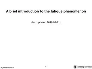
High Cycle Fatigue (HCF) analysis (last updated 2011-09-27)
Aim For small loadings/long lives (with respect to the number of load cycles), fatigue life calculations are generally stress-based. The aim of this presentation is to give a short introduction to stress-based High Cycle Fatigue (HCF) analysis.
Basic observations; Wöhler-diagrams/SN-curves Experiments made on smooth test specimens result in stress-life curves (so called SN-curves) of the type shown below (such diagrams are also referred to as Wöhler-diagrams) Fatigue limit (or Endurance limit), “utmattningsgräns” in Swedish No. of cycles to failure No. of load reversals to failure In the region of longer lives, the curve may often be described bythe following relation Basquin’s relation For some materials a true fatigue limit exists, while for others it is defined as the stress for which the material can withstand a certain (large) number of load cycles, say 1E6 or 1E7.
Wöhler-diagrams/SN-curves; cont. • Note that • The fatigue limit could for a mild steel be in the order of 140 MPa • There is often a large scatter in fatigue data; thus the SN-curve represents the mean behavior • Aluminum is a material that lacks a fatigue limit • Basquin’s relation is sometimes rewritten in the following way
Mean stress effects Experiments reveal that the mean stress has a marked effect on the fatigue life of uniaxially loaded specimens, while it has a much weaker influence on specimens loaded in pure torsion. Basically, a positive mean stress decreases the fatigue life. In what follows we will concentrate on the case of a positive mean stress. In order to fully describe this kind of behavior, we note that we are to deal with a relation between three quantities, namely the stress amplitude σa, the mean stress level σmand the fatiguelifeNf, which for instancemay be written However, such a relation will (for each material in each specific condition) require an enormous amount of test data to set up. Now, since we when adopting a so called total life approach (not distinguishing between different stages of the fatigue process) generally are interested in infinite life, the life variable becomes a parameter (a chosen large value, 1E6 or 1E7). Thus
Mean stress effects; cont. Mean stress effects; cont. From the previous slide we have The most widely used relations of this type are One may note that all three of the relations to the left can be cast in the following form Soderberg’s relation Goodman’s relation Gerber’s relation where σ0 is a reference stress (the yield stress or the ultimate tensile stress) while m is a parameter.
Mean stress effects; cont. Mean stress effects; cont. For a mild steel we get the following form for the Soderberg, Goodman and Gerber relations, resp. Soderberg’s relation Goodman’s relation Gerber’s relation Experiments seem to indicate that the true response typically can be found in between the Goodman and the Gerber curves, and that the usage of the former thus provides a conservative approach.
The Haigh-diagram Instead of proposing one single function describing the amplitude stress as a function of the mean stress (for infinite life) as done above, one may of course use a multi-linear function. One such example is the so called Haigh-diagram, see below. Data for the same mild steel as discussed above. In addition to the fatigue/endurance limit σfl on the ordinate (for an alternating loading), and the ultimate tensile strength σutson the abscissa (for a static loading), one also uses experimental data for a pulsating loading.
The Haigh-diagram; cont. • Note that • No distinction is made between different fatigue stages (i.e. crack initiation and crack propagation) in the Wöhler- and Haigh-diagrams. Therefore, we refer to analyses based on these as examples oftotal life approaches to fatigue design. • The Haigh-diagram allows, in its standard form, only design with respect to infinite life. • Values for σfl and σflp are generally recorded for uniaxial loading, bending and torsional loading. • The reason why only two combinations of σa and σm are used in the Haigh-diagram is the economical- and time cost of performing fatigue experiments.
The Haigh-diagram; cont. Sometimes a line representing the yield limit is included in the Haigh-diagram, since plastic flow is to be avoided. Data for the same mild steel as discussed above.
Topics still not discussed Topics for the next lecture It is important to note that the material response found in material tables etc is found for laboratory specimens tested at laboratory conditions. For industrial/real life applications the fatigue data and/or working point must be adjusted, and this will be one of the topics for the next lecture. Furthermore, in real life applications the loading will most likely not be as simple as an oscillating one. Thus, on the next lecture the most widely used cycle count method, the so called Rain Flow Count method, will be presented (multi-axial fatigue will briefly be discussed later on).