Zoology 2005 Part 2
Zoology 2005 Part 2 Richard Mott Inbred Mouse Strain Haplotype Structure When the genomes of a pair of inbred strains are compared, we find a mosaic of segments of identity and difference (Wade et al, Nature 2002).

Zoology 2005 Part 2
E N D
Presentation Transcript
Zoology 2005 Part 2 Richard Mott
Inbred Mouse Strain Haplotype Structure • When the genomes of a pair of inbred strains are compared, • we find a mosaic of segments of identity and difference (Wade et al, Nature 2002). • A QTL segregating between the strains must lie in a region of sequence difference. • What happens when we compare more than two strains simultaneously?
No Simple Haplotype Block Mosaic Yalcin et al 2004 PNAS
In-silico Mapping • Simple idea- • Collect phenotypes across a set of inbred strains • Genotype the strains (ONCE) • Look for phenotype-genotype correlation • Works well for simple Mendelian traits (eg coat colour) • Suggested as a panacea for QTL mapping
In-silico Mapping Problems • Less well-suited for complex traits • Number of strains required grows quickly with the complexity of the trait. Suggested at least 100 strains required, possibly more if epistasis is present • Require high-density genotype/sequence data to ensure identity-by-state = identity by-descent • May be very useful for the dissection of a QTL previously identified in a F2 cross (look for patterns of sequence difference)
Recombinant Inbred Lines • Panels of inbred lines descended form pairs of inbred strains • Genomes are inbred mosaics of the founders • Lines only need be genotyped once • Similar to in-silico mapping except • identity-by-descent=identity-by-state • Coarser recombination structure • ?lower resolution mapping?
Testing if a variant is functional without genotyping it(Yalcin et al, Genetics 2005) • Requirements: • A Heterogeneous Stock, genotyped at a skeleton of markers • The genome sequences of the progenitor strains • A statistical test
Merge Analysis • Each polymorphism groups together the founders according to their alleles • If the polymorphism is functional, then a model in which the phenotypic strain effects are estimated after merging the strains together should be as good as a model where each strain can have an independent effect. • Compare the fit of “merged” and “unmerged” genetic models to test if the variant is functional. • If the fit of the merged model is poor then that variant can be eliminated.
How can we show a gene under a QTL peak affects the trait? • Genetic Mapping identifies Functional Variants, not Genes • Could be a control element affecting some other gene
Quantitative Complementation KO wt Low High 30 0 50 100
Quantitative Complementation KO wt Low High d 30 0 50 100
Quantitative Complementation KO wt Low High d d 30 0 50 100 D= d -d
Quantitative Complementation KO wt Low High d d 30 0 50 100 D= d -d
Using Functional Information to Confirm Genes • Further experiments • further bioinformatics, eg networks, functional annotation (GO, KEGG) • candidate gene sequencing • gene expression analyses (eQTL) of • founder strains • HS
Enhancer reporter assays enhancer promoter luciferase reporter enhancer promoter luciferase reporter
Large-Scale Genetic Mapping • Using a Heterogeneous Stock • Multiple Phenotypes collected in parallel
Predictions (from simulation of an HS population) • In a population of 1,000 HS animals: • Genome-wide power to detect 5% QTL ~ 0.92 • Resolution < 2 Mb
Study design • 2,000 mice • 15,000 diallelic markers • More than 100 phenotypes • each mouse subject to a battery of tests spread over weeks 5-9 of the animal’s life • more (post-mortem) phenotypes being added
Covariates • For each phenotype, we recorded covariates, eg, • experimenter • time of day • apparatus (eg, Shock Chamber 3)
Data collection • All animals microchipped • Automated data checking, processing and uploading • All data uploaded into the Integrated Genotyping System (IGS) database
Genotypes from Illumina • Genotyped and phenotyped 2,000 offspring • Genotyped 300 parents • Pedigree analysis shows genotyping was 99.99% accurate • 11, 558 markers polymorphic in HS
QTL mapping • Models • HAPPY and single marker association • Fitting framework • Linear regression of (transformed) phenotypes • Survival analysis for latency data • Logit-based models for categorical data • Significant covariates incorporated into the null model, eg Null = Startle ~ TestChamber + BodyWeight + Year + Age + Hour + Gender Additive Null + additive genetic info for locus Full Null + full genetic info for locus
QTL mapping • Significance tests • partial F-test (linear models), Chi-square / LRT (others) • Significance thresholds • different for each phenotype • have to take into account LD • fit distribution to scores of permuted data
E-values • We set score thresholds using ideas from sequence databank search programs such as BLAST
E-values • We set score thresholds using ideas from sequence databank search programs such as BLAST • The E-value of a threshold is the number of times you would expect to see a false positive exceed the threshold in a genome scan
E-values • We set score thresholds using ideas from sequence databank search programs such as BLAST • The E-value of a threshold is the number of times you would expect to see a false positive exceed the threshold in a genome scan • Applying the Bonferroni correction to the number of marker intervals is too severe because LD makes neighbouring scores correlated.
E-values • We set score thresholds using ideas from sequence databank search programs such as BLAST • The E-value of a threshold is the number of times you would expect to see a false positive exceed the threshold in a genome scan • Applying the Bonferroni correction to the number of marker intervals is too severe because LD makes neighbouring scores correlated. • Permutation analyses indicate the score of the most significant expected random score amongst all ~12000 marker intervals behaves as if it was drawn from M~4000 independent tests.
E-values • We set score thresholds using ideas from sequence databank search programs such as BLAST • The E-value of a threshold is the number of times you would expect to see a false positive exceed the threshold in a genome scan • Applying the Bonferroni correction to the number of marker intervals is too severe because LD makes neighbouring scores correlated. • Permutation analyses indicate the score of the most significant expected random score amongst all ~12000 marker intervals behaves as if it was drawn from M~4000 independent tests. • Hence a nominal P-value of p corresponds to an E-value of pM
Problems Our population includes both siblings and unrelateds • We have ignored this distinction And therefore: • Confounding environmental family effects with genetic family effects • Allowing ghost peaks due to linkage disequilibrium between markers within a sibship Our solution so far: (1) Investigating the effect of environmental factors and building covariates into the model (2) Identify peaks by a multiple conditional fit
Multiple Peak FittingForward Selection • For each phenotype’s genome scan: • Make list of all peaks > genome-wide threshold T • Fit most significant peak, P1 • Go through list of peaks, refitting each on conditional upon the most significant peak. • Add the most significant remaining peak, P2 • Continue refitting remaining peaks P3 , P4 … and adding them into model until the most significant remaining peak < T
Peaks found by multiple conditional fit Multiple conditional fit (using additive model only) number of phenotypes
Database for scans Additive model Full model • E-value thresholds • additive only • E<0.01 is about the same as genome-wide corrected p<0.01.
Database for scans zoom in
QTL Mapping: Validation • Coat colour • Detection of known QTLs
A known QTL: HDL HS mapping Wang et al, 2003
New QTLs: two examples • Freeze.During.Tone (from Cue Conditioning behavioural experiment) …………1 peak • % of CD4 in CD3 cells (immunology assay) …………10 peaks
Freezing TONE TONE Cue Conditioning • Freezing in response to a conditioned stimulus
Cue Conditioning • Freeze.During.Tone: huge effect, small number of genes chr15 cntn1: Contactin precursor (Neural cell surface protein)