Download

1 / 24
250 likes | 733 Views
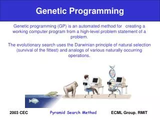
Genetic Programming Chapter 6 G P quick overview Developed: USA in the 1990’s Early names: J. Koza Typically applied to: machine learning tasks (prediction, classification…) Attributed features: competes with neural nets and alike needs huge populations (thousands) slow Special:

E N D
Genetic Programming Chapter 6
GP quick overview • Developed: USA in the 1990’s • Early names: J. Koza • Typically applied to: • machine learning tasks (prediction, classification…) • Attributed features: • competes with neural nets and alike • needs huge populations (thousands) • slow • Special: • non-linear chromosomes: trees, graphs • mutation possible but not necessary (disputed; probably true if population sizes are very very large)
Introductory example: credit scoring • Bank wants to distinguish good from bad loan applicants • Model needed that matches historical data
Introductory example: credit scoring • A possible model: IF (NOC = 2) AND (S > 80000) THEN good ELSE bad • In general: IF formula THEN good ELSE bad • Only unknown is the right formula, hence • Our search space (phenotypes) is the set of formulas • Natural fitness of a formula: percentage of well classified cases of the model it stands for --- be aware if over-fitting: evaluating the model on unseen examples should be a better approach. • Natural representation of formulas (genotypes) is: parse trees
AND = > NOC 2 S 80000 Introductory example: credit scoring IF (NOC = 2) AND (S > 80000) THEN good ELSE bad can be represented by the following tree
Tree based representation • Trees are a universal form, e.g. consider • Arithmetic formula • Logical formula • Program (x true) (( x y ) (z (x y))) i =1; while (i < 20) { i = i +1 }
Tree based representation (x true) (( x y ) (z (x y)))
Tree based representation i =1; while (i < 20) { i = i +1 }
Tree based representation • In GA, ES, EP chromosomes are linear structures (bit strings, integer string, real-valued vectors, permutations) • Tree shaped chromosomes are non-linear structures • In GA, ES, EP the size of the chromosomes is fixed • Trees in GP may vary in depth and width
Tree based representation • Symbolic expressions can be defined by • Terminal set T • Function set F (with the arities of function symbols) • Adopting the following general recursive definition: • Every t T is a correct expression • f(e1, …, en) is a correct expression if f F, arity(f)=n and e1, …, en are correct expressions • There are no other forms of correct expressions • In general, expressions in GP are not typed (closure property: any f F can take any g F as argument)
Offspring creation scheme Compare • GA scheme using crossover AND mutation sequentially (be it probabilistically) • GP scheme using crossover OR mutation (chosen probabilistically) --- this is anyway the schema Dr. Eick recommends for almost all EC-stystems
GA flowchart GP flowchart
Mutation • Most common mutation: replace randomly chosen subtree by randomly generated tree
Mutation cont’d • Mutation has two parameters: • Probability pm to choose mutation vs. recombination • Probability to chose an internal point as the root of the subtree to be replaced • Remarkably pm is advised to be 0 (Koza’92) or very small, like 0.05 (Banzhaf et al. ’98) • The size of the child can exceed the size of the parent
Recombination • Most common recombination: exchange two randomly chosen subtrees among the parents • Recombination has two parameters: • Probability pc to choose recombination vs. mutation • Probability to chose an internal point within each parent as crossover point • The size of offspring can exceed that of the parents
Parent 1 Parent 2 Child 1 Child 2
Selection • Parent selection typically fitness proportionate • Over-selection in very large populations • rank population by fitness and divide it into two groups: • group 1: best x% of population, group 2 other (100-x)% • 80% of selection operations chooses from group 1, 20% from group 2 • for pop. size = 1000, 2000, 4000, 8000 x = 32%, 16%, 8%, 4% • motivation: to increase efficiency, %’s come from rule of thumb • Survivor selection: • Typical: generational scheme (thus none) • Recently steady-state is becoming popular for its elitism
Initialization • Maximum initial depth of trees Dmax is set • Full method (each branch has depth = Dmax): • nodes at depth d < Dmax randomly chosen from function set F • nodes at depth d = Dmax randomly chosen from terminal set T • Grow method (each branch has depth Dmax): • nodes at depth d < Dmax randomly chosen from F T • nodes at depth d = Dmax randomly chosen from T • Common GP initialisation: ramped half-and-half, where grow & full method each deliver half of initial population
Bloat • Bloat = “survival of the fattest”, i.e., the tree sizes in the population are increasing over time • Ongoing research and debate about the reasons • Needs countermeasures, e.g. • Prohibiting variation operators that would deliver “too big” children • Parsimony pressure: penalty for being oversized
Problems involving “physical” environments • Trees for data fitting vs. trees (programs) that are “really” executable • Execution can change the environment the calculation of fitness • Example: robot controller • Fitness calculations mostly by simulation, ranging from expensive to extremely expensive (in time) • But evolved controllers are often to very good
Example application: symbolic regression • Given some points in R2, (x1, y1), … , (xn, yn) • Find function f(x) s.t. i = 1, …, n : f(xi) = yi • Possible GP solution: • Representation by F = {+, -, /, sin, cos}, T = R {x} • Fitness is the error • All operators standard • pop.size = 1000, ramped half-half initialisation • Termination: n “hits” or 50000 fitness evaluations reached (where “hit” is if | f(xi) – yi | < 0.0001)
Discussion Is GP: The art of evolving computer programs ? Means to automated programming of computers? GA with another representation?