Download

1 / 36
360 likes | 509 Views
This presentation explores advanced methodologies for 3D Non-LTE (NLTE) analysis in large stellar surveys, particularly for galactic archaeology. We discuss recent progress in 1D and 3D LTE/NLTE analyses, calibration techniques, and practical implementations for analyzing over 1 million FGK stars. Key findings highlight the significance of NLTE in resolving discrepancies in chemical abundance measurements. We also present case studies on magnesium and calcium line formation, demonstrating the crucial role of NLTE in enhancing the accuracy of stellar parameter estimations.

E N D
3D and NLTE analysis for large stellar surveys Karin Lind Uppsala University, Sweden Martin Asplund, Paul Barklem, AndreyBelyaev, Maria Bergemann, Remo Collet, Zazralt Magic, Anna Marino, Jorge Meléndez, Yeisson Osorio
Outline • Introduction • 1D LTE/NLTE • Worst-case scenarios • Recent progress • Calibration techniques • Practical implementation • Applications • 3D LTE/NLTE • Worst-case scenarios • Observational tests • Mg : 1D/<3D>/LTE/NLTE • Ca : 1D/<3D>/3D/LTE/NLTE • Applications
Motivation • Galactic archaeology by chemical tagging of FGK stars • Statistics : Soon > 106 stars • Precision(S/N, wavelength range) : • σ[X/H] < 0.1dex, σTeff<150K, σlog(g)<0.3dex • Accuracy(assumptions: 1D, LTE, atomic data) : • σ[X/H]< 0.5 dex, σTeff<400K, σlog(g)< 1 dex
Methods Model atmosphere Detailed rad. Transfer 1D/<3D>/3D LTE 1D/3D LTE/NLTE R. Collet
(1D) N- Is it really necessary? Is it safe?
Worst-case scenario I NaD lines in metal-poor horisontal branch stars Lind et al. 2011, Marino et al. 2011 B-I
Worst-case scenario II OI 777nm triplet at very low metallicities LTE trend Fabbian et al. 2009
Input data for NLTE analysis Energy levels + oscillator strengths + photo-ionization cross sections Red boxes : have sufficient(?) data Blue boxes : missing e.g. QM photo-ionisation, but NLTE still attempted
Input data for NLTE analysis Blue boxes : QM hydrogen collisions exist or will exist
Input data for NLTE analysis Most important free parameter in NLTE modelling of Fe is FeI+HI collisional cross-section Black – LTE Blue – NLTE with no hydrogen collisions Solar neighborhood MDF Halo MDF [X/Fe] vs [Fe/H]
Calibration techniques: ionisation balance Korn et al. 2003 FeI/FeIIionisation equilibrium calibrated using Hipparcos gravities S(H)=3
Calibration techniques: excitation balance Bergemann & Gehren 2008 “Thus, NLTE can solve the discrepancy between the abundances derived from the MnI resonance triplet at 403 nm and excited lines, which is found in analyses of metal-poor subdwarfs and subgiants” S(H)=0.05
Calibration techniques: CLV Allende Prieto et al. (2004) Solar centre-to-limb variation of OI lines
Practical implementation I “Curves-of-growth” from UV-NIR: 3200 FeI lines 107FeII lines Teff=6500K log(g)=4.0 ξ=2km/s ΔNLTE Lind et al. (2012)
Practical implementation II Pre-computed departure coefficients NLTE synthesis T. Nordlander
FeI NLTE grid Lind et al. (2012)
Application : metal-poor stars LTE NLTE +PHOT Ruchti et al. (2012)
Application : metal-poor stars LTE NLTE+PHOT Serenelli et al. (2013)
3D (LTE/NLTE) Is it really necessary? Is it safe?
Stagger grid Magic et al. 2014
Abundance patterns Keller et al. (2014) Dashed –200 Msun PISN Solid – 60Msun fallback 3D N-LTE
Worst-case scenario III Li isotopic abundances 3D N-LTE Lind et al. 2013 Asplund et al. 2006
Observational tests: the Sun Pereira et al. 2013 “We confronted the models with observational diagnostics of the [solar] temperature profile: continuum centre-to-limb variations (CLVs), absolute continuum fluxes, and the wings of hydrogen lines. We also tested the 3D models for the intensity distribution of the granulation and spectral line shapes. ” “We conclude that the 3D hydrodynamical model is superior to any of the tested 1D models.”
Observational tests: low [Fe/H] Klevas et al. 2013 FeI line assymmetries in the metal-poor giant HD122563
1.5/3D + NLTE LiI : Asplund et al. 2003, Sbordone et al. 2010 OI, FeI : Shchukina et al. 2005 OI : Pereira et al. 2010, Prakapavičius et al. 2013 LiI, NaI, CaI: Lind et al. 2013
Mg b in a VMP SG “No” free parameters! HD140283 Teff=5780K log(g)=3.7 [Fe/H]=-2.4 1D LTE 1D NLTE <3D> LTE <3D> NLTE Yeisson Osorio
Ca in a VMP dwarf 1D NLTE LTE 3D <3D> HD19445 Teff=6000K log(g)=4.5 [Fe/H]=-2.0
Ca in a VMP dwarf 1D NLTE LTE 3D <3D> HD19445 Teff=6000K log(g)=4.5 [Fe/H]=-2.0
Ca in a EMP TO Start ? Goal G64-12 Teff=6430K log(g)=4.0 [Fe/H]=-3.0 Bullets: Optical CaI lines Squares: NIR CaII triplet
Ca in a EMP TO Start ? Goal Bullets: Optical CaI lines Squares: NIR CaII triplet
Ca in a EMP TO Start ? Goal Bullets: Optical CaI lines Squares: NIR CaII triplet
Ca in a EMP TO Start ? Goal Bullets: Optical CaI lines Squares: NIR CaII triplet
Ca in a EMP TO Start ? Goal Bullets: Optical CaI lines Squares: NIR CaII triplet
Ways forward A : NLTE-sensitive, B : not NLTE-sensitive