IGS Time Scale Algorithm: Results & Enhancements
Explore the results and improvements of the new IGS Time Scale Algorithm presented at the 2009 AGU Fall Meeting. Learn about clock measurements, algorithm features, enhanced stability, and clock modeling.

IGS Time Scale Algorithm: Results & Enhancements
E N D
Presentation Transcript
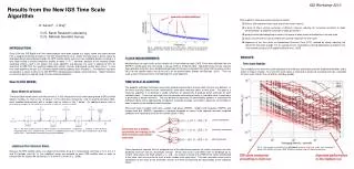
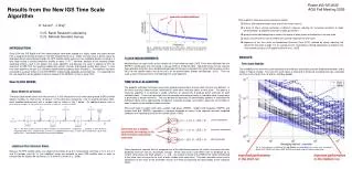
Poster #G11B-0632 AGU Fall Meeting 2009 Results from the New IGS Time Scale Algorithm K. Senior†, J. Ray‡ † U.S. Naval Research Laboratory‡ U.S. National Geodetic Survey peaks at N x (2.0029 ± 0.0005) cpd CLOCK MEASUREMENTS Measurements of each clock’s phase relative to a fixed reference clock (GPS Time) were obtained from the REPRO1 combination over the period 1 January 2006 to 15 March 2006. Tabulated at five-minute intervals these geodetic estimates are a weighted combination of estimates submitted from up to 9 IGS analysis centers (ACs) for the satellite clocks and up to 6 ACs for the ground clocks [Kouba and Springer, 2001]. They are used as input measurements in the following time scale algorithm. TIME SCALE ALGORITHM The geodetic estimation technique necessarily produces observations of each clock that are rank deficient in the sense that each clock must be referenced to some other reference clock, or time scale. The goal of a timescale algorithm is to generate a stable reference, or equivalently to produce better estimates of each individual clock. These are equivalent since for example estimating perfectly an individual clock is equivalent to generating a perfect reference. The rank deficiency represents an observability problem in estimating the individual clocks and is addressed by introducing “ensemble average” assumptions about the set of clocks in order to constrain the individual clock estimation. Since each type of random walk input—random walk phase (RWPH), random walk frequency (RWFR), and random walk drift (RWDR)—represents a separate ensemble of noises, three separate recursive weighted conditions are imposed to constrain the solution [Stein, 1993]: These constraints stipulate that the weighted sum of the differences between the clocks’ true states and their predicted states be zero on (ensemble) average. Since each clock’s state differs from its prediction by its random noise inputs, the clock weights ai, bi, and ci are chosen inversely to the RMS of the noises contributing to that state, that is inverse to the level of each random walk noise input. This both normalizes each clock’s contribution to the noise of the ensemble and has the effect of improving the observability of the individual clocks. • Other algorithm features and enhancements include: • Kalman filter implementation (also true for the earlier version) • a bank of filters running nominally at different intervals, allowing for increased sensitivity to clock break detection & adaptive estimation of clock parameters • graceful outlier downweighting to reduce the impact of clock events or bad data on the time scale • clocks may enter/leave the ensemble with minimal impact on the time scale • alignment of the time scale to Coordinated Universal Time (UTC) realized by slowly adjusting the drift of the timescale to align it to an average of UTC realizations at timing laboratories (included in the IGS network) using an LQG algorithm [Senior et al., 2003] INTRODUCTION Since 2004 the IGS Rapid and Final clock products have been aligned to a highly stable time scale derived from a weighted ensemble of clocks in the IGS network [Senior et al., 2003]. The time scale is driven mostly by Hydrogen Maser ground clocks though the GPS satellite clocks also carry non-negligible weight, resulting in a time scale having a one-day frequency stability of about . However, because of the relatively simple weighting scheme used in the legacy time scale algorithm and because the scale is aligned to UTC by steering it to GPS Time the resulting stability over shorter intervals and beyond several days suffers. A new time scale algorithm (version 2.0) has been implemented to address these limitations. The algorithm has been evaluated to a subset of data in the IGS REPRO1 reprocessing campaign, presented here. It is expected that the new algorithm will be applied in the final release of the REPRO1 results in early 2010. New CLOCK MODEL Basic Model for all Clocks The basic clock model used in the new (version 2.0) IGS timescale for each clock (both ground & GPS satellite clocks) includes the clock’s time (or phase), its first derivative (frequency), and its second derivative (drift), each modeled stochastically with a random walk as shown in Fig. 1 below. An additional phase state is included to model a pure white phase noise as well as harmonic terms. Additional Pure Harmonic States Because the GPS satellite clocks are subject to harmonics of up to 2 nanoseconds nominally at 12-h, 6-h, 4-h and 3-h periods (see Fig. 2), four additional states are included for each GPS satellite clock in order to compensate the largest two harmonics (12-h and 6-h) [ Senior et al., 2008] . Fig. 2. Amplitude spectrum for the GPS clocks. Spectra were calculated individually for each satellite and averaged over the entire constellation of clocks. RESULTS Time Scale Stability The instability of the new time scale compared to the old was calculated using the Hadamard deviation and is shown in Figure 3 below. The new time scale (blue) is improved at almost all averaging intervals, especially for times much shorter than 1d and for multi-day periods. phase constraints Each clock has 3 weights, dynamically set inversely to the level of random walk driving each state Fig. 1. The basic model used for all clocks includes the clock’s phase, x, frequency, y, and drift, d, each driven by integrated white noises (random walks) as well as an additional phase state, , necessary to model also a pure white phase noise. Up to two pure harmonics may also be included. frequency constraints drift constraints Fig. 3 The frequency instability of the old (black) and new (blue)time scales over the period 3 March (MJD 53800) to 3 August 2006 (53950) calculated using the Hadamard deviation. improved performance in the short run improved performance in the medium run
Sample Filter Outputs Fig. 4 Filter output (above) for the clock “ONSA” at Onsala over the period 10 January to 6 March 2006. The filter phase (gray and black), frequency (red), and drift (blue)states are shown in the top panel, all referenced to the steered IGS timescale. The middle panel shows corresponding state sigmas, while the bottom panel shows the clock weights used in the timescale. A separate polynomial has been removed from each time series in the top panel, its value shown in the legend. The legend also shows any phase or frequency breaks detected/removed during filtering. Note that for this very stable clock, the phase state with white noise and harmonics (black) is indistinguishable from the simple phase estimate (gray). Fig. 5 Filter output for the GPS satellite clock for PRN11 over the period 1 to 21 May 2006. The filter phase (gray and black), frequency (red), and drift (blue)states are shown in the top panel, all referenced to the steered IGS timescale. The middle panel shows corresponding state sigmas, while the bottom panel shows the clock weights used in the timescale. A separate polynomial has been removed from each time series in the top panel, its value shown in the legend. The legend also shows any phase or frequency breaks detected/removed during filtering. Note that for this satellite clock possessing strong periodic variations near 12h and 24h, that the phase state with white noise and harmonics (black) differs noticeably from the simple phase estimate (gray). REFERENCES Senior K., Ray J., Beard R., Characterization of periodic variations in the GPS satellite clocks, GPS Solutions, DOI 10.1007/s10291-008-0089-9, 2008. Kouba J., Springer T., New IGS station and satellite clock combination. GPS Solutions 4:31–36, 2001. Senior K., Koppang P., Ray J., Developing an IGS time scale. IEEE Trans Ultrason Ferroelectr Freq Control 50:585–593, 2003. Stein, S. R. , Advances in time-scale algorithms, Proc. of the 24th Annual Precise Time & Time Interval (PTTI) Applications and Planning Meeting, Greenbelt, Maryland, 289—303, 1993. Alignment to UTC Fig. 6 Estimates (right) over 150 d of the new time scale versus UTC using an average of several calibrated timing lab sites.