Download
1 / 29
290 likes | 486 Views
Bayesian Doubly Optimal Group Sequential Design for Clinical Trials. Goal : Beat the frequentists at their own game in phase III clinical trial design. Requirements: Maintain overall false-positive error rate and targeted power

E N D
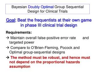
Bayesian Doubly Optimal Group Sequential Design for Clinical Trials Goal: Beat the frequentists at their own game in phase III clinical trial design • Requirements: • Maintain overall false-positive error rate and targeted power • Compare to O’Brien-Fleming, Pocock and Optimal group-sequential designs • The method must be robust, and hence must not depend on the proportional hazards assumption
Solution: A Bayesian Doubly Optimal Group Sequential (BDOGS) Design (Wathen and Thall, Stat in Medicine, 2008) • A robust Bayesian decision-theoretic approach to designing group sequential clinical trials 2. The focus is on two-arm trials with time-to-failure (TTF) outcomes 3. Uses Bayesian adaptive model selection 4. Maintains overall frequentist size and power
1) Assume the data come from one of M models (characterized by their hazard functions) 2) Before the trial:Derive the Optimal Decision Bounds for each model,and store them 3) During the trial:At each interim analysis, make decisions using the Optimal Decision Bounds of the Optimal Model 4) The optimal boundaries depend on the model, and the model is optimized adaptively The decision boundaries may change from one interim evaluation to the next Basic Elements of BDOGS BDOGSillustration
A Doubly Optimal Procedure Step 1 (Before the Trial):For each of M specific models, obtain the Optimal Decision Boundaries using forward simulation. Step 2 (During the Trial):Obtain posterior model probabilities for the set of M possible models using approximate Bayes Factors to determine the OptimalModel. Step 3 (During the Trial):Apply the optimal decision boundaries corresponding to the optimal model at each interim decision based on the most recent data.
d= mE – mS = actual improvement in median failure time of experimental (E) over standard (S), a parameter under the Bayesian model (hence random) d* = fixed desired improvement in median failure time of E over S Expected Utility = ½ Ed = 0(N) + ½ Ed = d*(N)
Decision Boundaries To facilitate computation, for each modelBDOGS uses the two parametric boundary functions PU = aU – bU { N+(Xn)/N } PL = aL + bL { N+(Xn)/N } whereN = maximum sample size, and N+(Xn) = # failure events in data Xn (aU , bU , cU , aL , bL , cL ) characterize the decision boundary for a given model cU cL
Decision Rules Superiority of S over E rS = Pr( d < -d* | x ) > PU Stop and select S Superiority of E over S rE = Pr( d > d* | x ) > PU Stop and select E Futility rS< PLandrE< PLStop for futility Acquire more information PL rS, rE PU Continue randomizing to obtain more information
Forward Simulation Simulate the entire trial 5000 times assuming d = 0, and 5000 times assumingd = d* : • For each interim analysis, calculaterEandrS, andstorerE, rS, and alsostore • [# of patients], [# events] for each treatment arm. 2. Applythe decision rule, dto obtain the expected utility for a trial usingd 3. Find dthat maximizes the expected utility. (A complex search algorithm is required.)
Examples of Hazard Functions (Models) Hazard function for M1 = exponential distribution is constant
A Metastatic Non-Small Cell Lung Cell Cancer (NSCLC) Trial Median overall survival (OS) in metastatic NSCLCis about 4 months A phase III trial of localized surgery or radiation therapy versus systemic chemotherapy for metastatic NSCLC was designed with the goal to improve median progression-free survival (PFS) from 4 to 8 months Initially, a conventional .05/.90 group sequential design with O’Brien-Fleming boundaries was planned, with up to 3 tests at 30, 60 and 89 events.
Under the “usual” assumptions, accruing 2 to 4 patients/month, a typical O’Brien-Fleming .05/.90 group sequential design will require ~ 100 to 120 patients and take ~ 2 ½ to 4 ½ years to complete
Analysis of Historical Data on PFS time in Metastatic NSCLS A preliminary goodness-of-fit analysis, based on a published Kaplan-Meier plot of PFS times of NSCLC patients with metastatic disease, showed that the Log Normal distribution gave a much better fit than the Weibull or Exponential. The proportional hazards assumption was very likely invalid. The hazard function was very likely non-monotone.
A BDOGS Design for the NSCLC Trial To test H0: d = 0 versus H1: d 0 Assume med(T) = 4 mos. for std. therapy Type I Error = .05, Power= 0.90 ford*= 4months, improvement to med(T) = 8 mos. Assume 2 patients per month accrual Up to5 interim analyses + 1 final analysis, at 25, 50, 75, 87, 112 and 122 events Five possible models
Possible Models (Hazard Functions) M1 = constant (Exponential model) M2 = increasing M3 = decreasing M4 = initially increasing, then a slight decrease M5 = initially increasing, then a large decrease A priori, the 5 models were assumed to be equally likely: Pr(M1) = …= Pr(M5) = .20.
Simulation Study for the NSCLS Trial • For comparability in the simulations: • An O’Brien-Fleming design was constructed to have the same 6 looks, for both superiority (reject the null) and inferiority (accept the null) decisions. • Both designs had the same maximum sample size N = 122 patients. • For each case (underlying true PFS distribution) studied, the data were simulated ahead of time and each method was presented with the same data.
Non-constant Hazards Used in Simulation Study for S (solid line) and E (dashed line)
Simulation Results: Null Case Lower - Upper Lines = 2.5 - 97.5 Percentiles Line in Box = Median Box = 25 – 75 Percentiles Dot in Box = Mean B = BDOGS, OF = O’Brien-Fleming
Simulation Results: Alternative Case Lower - Upper Lines = 2.5 - 97.5 Percentiles Line in Box = Median Box = 25 – 75 Percentiles Dot in Box = Mean B = BDOGS, OF = O’Brien-Fleming
Simulation Results If the hazard is constant, both BDOGS and OF maintain targeted size and power, but OF requires a much larger sample(33% to 51% more patients)
Simulation Results If the hazard is Log Normal, both BDOGS and OF maintain targeted size and power, but OF requires a much larger sample
Simulation Results If the hazard is Weibull, both BDOGS and OF maintain targeted power, BDOGS has a reduced size = .02, and OF requires a much larger sample
Simulation Results If the hazard is Weibull with decreasing hazard, BDOGS has size .07, OF has reduced power .81, and OF requires a much larger sample
Simulation Results If the hazard is Weibull with increasing hazard, both methods have greatly reduced size .01, OF has greatly increased power .99, and OF has a 61% to 141% larger sample size