The Primitive Roots
The Primitive Roots. Kelly Rae Murray Stephen Small Eamonn Tweedy Anastasia Wong. Our Goal: my’’+ cy’ + ky=0. Fit data into a model to estimate parameters at a certain confidence level Find problem areas in order to discover the best possible model Create a better model with our data.


The Primitive Roots
E N D
Presentation Transcript
The Primitive Roots Kelly Rae Murray Stephen Small Eamonn Tweedy Anastasia Wong
Our Goal: my’’+ cy’ + ky=0 • Fit data into a model to estimate parameters at a certain confidence level • Find problem areas in order to discover the best possible model • Create a better model with our data
The Experiment • A PZT patch was used to vibrate a metal beam. • The proximity sensor measured the vibrations of the beam. • The vibrations were recorded by computer software, creating a file giving us a graph of our data.
Truncating We found the maximum value of our data. This became the initial point for our graph. Set the time to begin at this point and end at 6 seconds. Oscillation Around Zero We found the mean of our graph, which initially was below zero. Then we shifted our data up to oscillate around zero. Before We can Model…
Fitting the Model • Guess and Check… • Start graphing with the same amplitude as our model • To oscillate with our model • Damp at the same rate as our model
Our Best Fit • For the Spring-Mass-Dashpot model… • C = c/m = -.7 • K = k/m = -1519.3 • These values were found by finding the q through the fminsearch code.
C=c/m 95% confidence (-.71732,-.68267) Standard Error =.008537 Sigma^2 = 1.0964e-010 K = k/m 95% confidence at (-1520.27,-1518.92) Standard Error = .333 Our Confidence IntervalsNon-Linear Least Square Results
Residuals Vs. Time Shows too much of a pattern. The periodicity tells us that there are modes that are not being represented. Seems to have a higher frequency at the beginning and end. Residuals Vs. Fitted Value Appears to be too much variation in the data. Should be random around zero. The higher spread at the beginning and end of the graph shows over-prediction and under-prediction Testing Our Residuals
QQ Plot • Comparing Error with Normal Distribution • Once again falls off at beginning and end. • This gives us enough proof that the Spring-Mass-Dashpot Model is not the best model for our experiment.
The Beam Model • Since this model is a PDE it accounts for higher modes not covered by the simpler model. • Hopefully, this model will give us a more accurate model for the motion of the beam.
Beam Model - Optimization • We first ran the beam simulation code without parameter optimization (fminsearch), using the ‘input’ data. The resulting fit didn’t quite match the latter portion of the data:
Beam Model - Optimization • Using some starting parameter guesses (conveniently close to those given to us), we ran an fminsearch that gave us a much closer fit to the actual data, even on the tail end:
Beam Model - Conclusion • The beam model provided a much closer fit to the data set. • The PDE model clearly gives us a much more realistic approximation of the beam’s vibration.