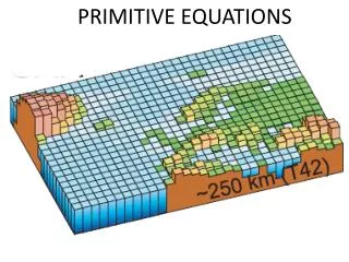
Primitive Equations
Primitive Equations. PRIMITIVE EQUATIONS. Definition. The so called primitive equations are those that govern the evolution of the large-scale motions. In other words, are the equations that describe the horizontal and vertical movement of the atmosphere and changes in temperature

Primitive Equations
E N D
Presentation Transcript
Primitive Equations PRIMITIVE EQUATIONS
Definition • The so called primitive equations are those that govern the evolution of the large-scale motions. • In other words, are the equations that describe the horizontal and vertical movement of the atmosphere and changes in temperature • They are easiest to interpret when we transform the z coordinate into p coordinate • that is: (x,y,z) -> (x,y,p)
Vertical movement in p-coordinates • The vertical velocity component in (x,y,p) coordinate is V- horizontal wind • Substituting (δp/ δz )=-ρg from the Hydrostatic equation: Note that w and ω have opposite sign: ascending (descending) movements ω negative (positive) ~ 1 week for a parcel to move from the lower to the upper troposphere 10hPa/day <<10hPa/day 100hPa/day
How to interpret ω Pressure ω=dp/dt 600mb 700mb 800mb 900mb 1000mb
Comparing w with ω • 100hPa/day is equivalent to 1km/day or 1cm/s in the lower troposphere and twice that value in the midtroposphere (see the example shown before) (the distance between two pressure levels increases with height)
Hydrostatic balance • We saw before (Joel’s classes) that the vertical component of the movement could be described as: • WhereCzare the vertical components of the Coriolis and Frictional forces, respectively • Vertical velocities are very small and we can assume to within ~1% that the upward gradient force balances the downward pull of gravity also for large-scale motions (this approach is not valid for cloud-scale motions though). • The Hydrostatic Balance can be assumed
Thermodynamic Energy Equation • The evolution of the weather systems is governed by dynamical (Newton’s Laws) AND THERMODYNAMIC PROCESSES (First and second law of thermodynamics) • The first law of the Thermodynamics (which represents changes and heat, expansion/contraction, increase/decrease in temperature, etc) is a prognostic equation for the parcel of air moving in the atmosphere • Changes in temperature cause changes in the gradient of geopotential height with implications for the winds (indicated by the relationships between pressure gradient and geopotential gradient)
First Law of Thermodynamics • The first Law of the Thermodynamics can be written as: • Where J represents the DIABATIC HEATING RATE (Joules kg-1 s-1 )and dt is the infinitesimal time interval. Dividing by dt and rearranging the terms we obtain: • Using the state equation for a substitution of αand replacing dp/dtbyωwe obtain the thermodynamic energy equation κ= R/cp=0.286
Interpretations • (1) Rate of change of temperature due to ADIABATIC EXPANSION OR COMPRESSION. • In a typical midlatitude disturbance, air parcels in the middle troposphere (~500hPa) undergo vertical displacements of ~100hPa/day. Assuming T~250K, the resulting adiabatic temperature change is: (1)
Interpretations • (2) represents the effects of DIABATIC heat sources and sinks: absorption of solar radiation, absorption/emission of longwave radiation, latent heat release and in the upper atmosphere, heat absorbed or liberated in chemical and photochemical reactions (as in the ozone layer) • Exchange of mass with the environment due to convection and turbulence can also affect (2) • Cancelations among these contributions occur throughout the atmosphere and the net radiative heating rates are less than 1o/day (2)
How horizontal advection and stability contribute to changes in Temperature • Let’s first expand the thermodynamic equation to let the horizontal advection appear explicitly (and separated from the vertical advection):
Interpretation • (i) Horizontal Advection term • (ii) combined effect of adiabatic compression and vertical advection • It can be shown (Ex. 7.37 ) by using the state equation and the fact that the adiabatic lapse rate Γd = g/cp and the environmental lapse rate is δT/ δT: (I) (II)
Let’s interpret these terms • If the observed lapse rate is equal to the dry adiabatic lapse rate then this term vanishes • In a stably stratified atmosphere, Γ < Γd and if there is subsidence (w<0 or ω>0) the contribution of this term is to increase temperature (+ contribution). The opposite occurs in ascending movements. The magnitude of this term depends on the stability of the layer (difference between Γ and Γd)
Other terms • If the motion is adiabatic and the atmosphere stably stratified then J=0 and parcels will conserve potential temperature as they move along their tridimensional trajectories
Example of the importance of advection of temperature in association with extratropical cyclones • Ex. 7.4 During the time that a frontal zone passes over a station the temperature falls at a rate of 2oC/h. The wind is blowing from the north at 40km/h and the temperature is decreasing with latitude at a rate of 10oC/100km. Estimate the terms in the eq. above, neglecting the Diabatic heating (i.e. J=0) y v Therefore, subsidence must be warming the air at a rate of 2oC/h as it moves southward! x
Tropical Regions: little variations in temperature from day to day
Weak temperature gradients Tropics: horizontal temperature gradients are much weaker than in the extratropics: horizontal advection is unimportant: temperatures at fixed points vary little from day to day Frontal systems ITCZ Anticyclone Anticyclone High temperature gradients Frontal systems
Tropical regions…Little variations in Daily Temperature Diabatic heating rates in regions of tropical convection (ex. Release of latent heat, absorption of solar radiation, etc) are larger than those in the extratropics. Ascents are concentrated in narrow rain bands: ITCZ. Warming due to the release of Latent Heat is compensated by cooling due to upward movement ITCZ Anticyclone Anticyclone
Tropical regions…Little variations in Daily Temperature δT/δp ~ moist adiabatic – which means that vertical movements in tropical regions that follow the moist adiabatic lapse rate do not add much to variations in temperature, even in regions where ω is negative and large (upward movement) In regions with slow subsidence (over tropical oceans), warming due to adiabatic compression is balanced by weak radiative cooling Slow Subsidence dominates Anticyclone Anticyclone
Inference of the vertical motion field: the continuity equation • Consider an air parcel shaped like a block with dimension δx, δy, δp. If the atmosphere is in hydrostatic balance, the mass of the block is not changing with time: • Divergence of horizontal wind
interpretation Northern Hemisphere Convergence at the surface due to frictional forces induces ascent Divergence at the surface due to frictional forces induces subsidence Vertical squashing Vertical stretching
Computation of vertical velocity • The vertical velocity at any given point (x,y) can be inferred diagnostically by integrating the continuity equation from some reference level p* to level p • We certainly need to know the horizontal wind field to solve this equation. • We can use a convenient reference level as the top of the atmosphere where p*=0 and ω=0. Integrating the above equation from the top down we obtain:
Pressure tendency • The equation for the pressure changes can be obtained by considering that:
Interpretations-1 (III) (I) (II) • At the surface, pressure tendency ~ 10hPa/day and the advections terms (II) and (III) are smaller. Therefore: Is the mass weighted vertically averaged divergence Considering ps ~ 1000hPa, 1day ~ 105 s ~ 10-7 s-1
Interpretation - 2 • We saw before that at some levels in the atmosphere ~ 10-6s-1. But the vertically averaged is 1 order smaller. This is because divergence changes sign for compensation between the lower and upper troposphere Z z Max -ω ~ 500hPa Max ω ~ 500hPa Div Div
ω in 500hPa (~ max) where divergence is ~0 July January
Solution of Primitive Equations • Primitive equations govern the evolution of the atmosphere and therefore are useful to forecast the weather and also for climate simulations. They are: HORIZONTAL MOTION 2 COMPONENTS u,v (PROGNOSTIC) HYPSOMETRIC EQUATION: DIAGNOSTIC F and J are expressed as functions of dependent variables (parameterized) THERMODYNAMIC ENERGY EQUATION (PROGNOSTIC) CONTINUITY BOTTOM BOUNDARY CONDITIONS
Numerical solutions Regularly spaced horizontal grid points at a number of vertical levels Δz t=0, u(x,y,p,t)= u(i,j,p,t) Δy Δx Equations involving horizontal and vertical derivatives are evaluated using finite difference techniques. Equations involving temporal derivatives.
Climate modeling • Climate models are systems of differential equations derived from the basic laws of physics, fluid motion, and chemistry formulated to be solved on supercomputers. For the solution the planet is covered by a 3-dimensional grid • http://www.oar.noaa.gov/climate/t_modeling.html
Regional models (mesoscale models) http://www.icess.ucsb.edu/asr/forecasts.htm
More applications and general circulation in the next lecture