Download
1 / 24
871 likes | 2.72k Views
Flood Estimation flood Control. Physical indications of past floods- flood marks and local enquiry Rational Method (CIA) Unit Hydrograph method Empirical methods Flood frequency methods. Empirical methods for Flood Estimation. Dicken’s formula Q=C*M^3/4 C= 11.4 for North India

E N D
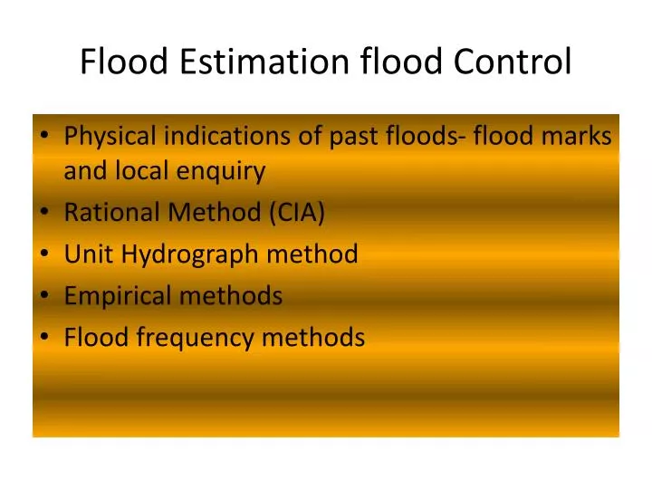
Flood Estimation flood Control • Physical indications of past floods- flood marks and local enquiry • Rational Method (CIA) • Unit Hydrograph method • Empirical methods • Flood frequency methods
Empirical methods for Flood Estimation • Dicken’s formula • Q=C*M^3/4 • C= 11.4 for North India • C= 13.9 to 19.5 for Central India • C= 22.5 to 25 for Western India • Ryve’s formula Q = CM ^(2/3) • Where C = varies from 6.8 to 15 kms • C = 6.75 if area is less than 24 kms from coast • C = 8.45 if area is 24 - 16 kms • C = 10.1 for hills • Q = Discharge in cumecs • M = Area in Sq. kms
Ali Nawaj Jung Bahadur’s formula • (0.993 - 1/14 Log A) • Q = CA • Value of C taken from 48 to 60 • This is applicable mainly in Deccan plains • A = Area of catchment in sq. km
Khoslas’ formula R = P - (T - 32)/3.74 Where T = mean temp F R & P are in cms. • Ingle’s formula Q=123*A/SQRT(A+10.4) • A= Area(sq.km) Englis gave the following formulae derived from data collected from 37 catchments in Bombay Presidency For Ghat areas R = 0.85 P - 30.5 Where R is run off in cms P = Precipitation cm For non Ghat areas R = {P - 17.8} x P/254
Barlow’ and Lacey have also given empirical formula as under R = KP Where R = Run off P = Precipitation K = Run off coefficient for different class of catchments like, A = Flat cultivated soil B = Flat partly cultivated C = Average D = Hills & plains with cultivation E = Very hilly areas Barlow has added another coefficient based on light rain, average rainfall with intermittent rains and continuous down pour etc. Lacey has given a formula as R = P ------------------ 1 + (304.8 F/PS) Where S = Catchment factor F = reservoir duration factor which is based on different classes as defined by Barlow’s equation.
Rational Method: In this method the basic equation which correlates runoff and rainfall is as follows Q = C * I * A Where Q = Runoff (Cubic meters per hour) C = Runoff Coefficient I = Intensity of rainfall in meters per hour A = Area of the drainage basin (Sq. Meters) Time of Concentration(Tc) is the time in hours taken by rain water that falls at the farthest point to reach the outlet of a catchment
The value of runoff coefficient C depends on the characteristics of the drainage basin such as soil type, vegetation, geological features etc. For different types of drainage basins the values of C are given below in table Table Value of C for different types of drainage basins
(unit hydrograph method) • Date hour Disch base rdinate ordinate • cumec flow dir -rf unit hyd • 12 aug 6 6 6 0 0 • 12 16 5 11 0.46 • 18 60 3.5 56.5 2.39 • 24 100 2.5 97.5 4.12 • 13 aug 06 68 3 65 2.75 • 12 35 4 31 1.31 • 18 11 4.5 6.5 0.27 • 24 7 5.5 1.5 0.06 • 14 aug 06 6 6 0 0
Flood frequency Average flood? Standard deviation? Coefficient of variation? Coefficient of Skewness Coefficient of flood Maximum flood for 100 year return period? Maximum flood for 500 year return period? Gumbel Method Log pearsonmethod
Flood frequency Gumbel Method • (P)=1-(e-e –y) T= 1/1-(e-e –y) Y(Reduced Variate)= (1/(0.78*σ))*(x-x¯+0.45 σ x=Flood magnitude with probability of occurrence, P Qt= Q¯+σ(0.78*ln (T)-0.45) for n> 50
Log Pearson Type III Distribution Cs’=Cs*((1+8.5)/N) Kz is read from tables Cs versus T Xt= Antilog of ZT Kz for different Return Period(T) & Cs
zT=Z¯+Kz*σz Cs’=Cs*((1+8.5)/N)
Results zT=Z¯+Kz*σz
Design Flood Estimation • Standard Project Flood (SPF) • Flood likely to occur. This is normally about 0.8 of MPF • Maximum Probable flood (MPF) • Maximum flood that can occur • Spillway design floods • Design Flood • The actual flood estimates for designing any structures
Special Projects Flood, GOG • Government of Gujarat Qspf= 0.8*a*C^b • a=29.0402 • b=0.9232 • C=Area (sq.Km)