Download

1 / 31
310 likes | 457 Views
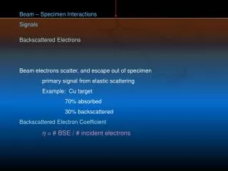
Beam – Specimen Interactions. Electron optical system controls: beam voltage (1-40 kV) beam current (pA – μ A) beam diameter (5nm – 1 μ m) divergence angle Small beam diameter is the first requirement for high spatial resolution Ideal: Diameter of area sampled = beam diameter

E N D
Beam – Specimen Interactions Electron optical system controls: beam voltage (1-40 kV) beam current (pA – μA) beam diameter (5nm – 1μm) divergence angle Small beam diameter is the first requirement for high spatial resolution Ideal: Diameter of area sampled = beam diameter Real: Electron scattering increases diameter of area sampled = volume of interaction
Scattering Key concept: Cross section or probability of an event Q = N/ntni cm2 N = # events / unit volume nt = # target sites / unit volume ni = # incident particles / unit area Large cross section = high probability for an event
From knowledge of cross sections, can calculate mean free path λ = A / N0ρ Q A = atomic wt. N0 = Avogadro’s number (6.02 x10²³ atoms/mol) ρ = density Q = cross section Smaller cross section = greater mean free path
Scattering (Bohr – Mott – Bethe) Types of scattering Elastic Inelastic Elastic scattering Direction component of electron velocity vector is changed, but not magnitude Ei Φe E0 Ei = E0 Ei = instantaneous energy after scattering Kinetic energy ~ unchanged <1eV energy transferred to specimen Target atom
Types of scattering Elastic Inelastic Inelastic scattering Both direction and magnitude components of electron velocity vector change Ei Φi E0 Ei < E0 Ei = instantaneous energy after scattering significant energy transferred to specimen Φi << Φe Target atom
Elastic scattering Electron deviates from incident path by angle Φc (0 to 1800) Results from interactions between electrons and coulomb field of nucleus of target atoms screened by electrons Cross section described by screened Rutherford model, and cross-section dependent on: atomic # of target atominverse of beam energy
Inelastic scattering • Energy transferred to target atoms • Kinetic energy of beam electrons decreases • Note: Lower electron energy will now increase the probability of elastic scattering of that electron • Principal processes: • Plasmon excitation • Beam electron excites waves in the “free electron gas” between atomic cores in a solid • 2) Phonon Excitation • Excitation of lattice oscillations (phonons) by low energy loss events (<1eV) - Primarily results in heating
Inelastic scattering processes 3) Secondary electron emission Semiconductors and insulators Promote valence band electrons to conduction band These electrons may have enough energy to scatter into the continuum In metals, conduction band electrons are easily energized and can scatter out Low energy, mostly < 10eV 4) Continuum X-ray generation (Bremsstrahlung) Electrons decelerate in the coulomb field of target atoms Energy loss converted to photon (X-ray) Energy 0 to E0 Forms background spectrum
Background = continuum radiation Inelastic scattering processes 5) Ionization of inner shells Electron with sufficiently high energy interacts with target atom Excitation Ejects inner shell electron Decay (relaxation back to ground state) Emission of characteristic X-ray or Auger electron
Total scattering probabilities: 107 Elastic events dominate over individual inelastic processes 106 Elastic Total cross section (g cm-1) Plasmon 105 Conduction L-shell 104 0 5 10 15 Electron energy (keV)
Max Born (1882-1970) -1926 Schrödinger waves are probability waves. The theory of atomic collisions. Bethe then uses Born’s quantum mechanical atomic collision theory as a starting point. He ascertained the quantum perturbation theory of stopping power for a point charge travelling through a three dimensional medium. Bethe ends up developing new methods for calculating probabilities of elastic and inelastic interactions, including ionizations. Found sum rules for the rate of energy loss (related to the ionization rate). From this, you can calculate the resulting range and energy of the charged particle, and with the ionization rate, the expected intensity of characteristic radiation.
From first Born approximation: Bethe’s ionization equation – the probability of ionization of a given shell (nl) ψp1 ψp E0 = electron voltage Enl = binding energy for the nl shell Znl = number of electrons in the nl shell bnl= “excitation factor” cnl = 4Enl / Bnl (B is an energy ~ ionization potential) { Bethe parameters ψ1s ψp2 Kα K L M
Optimum overvoltage = 2-3x excitation potential Binding energy = critical excitation potential This is an expression of X-ray emission, so as X-ray production volume occurs deeper at higher kV, proportionally more absorbed…
There are a number of important physical effects to consider for EPMA, but perhaps the most significant for determination of the analytical spatial resolution is electron deceleration in matter… Rate of energy loss of an electron of energy E (in eV) with respect to path length, x: dE / dx
Low ρ and ave Z High ρ and ave Z
Bethe’s remarkable result: stopping power… E = electron energy (eV) x = path length e = 2.718 (base of ln) N0 = Avogadro constant Z = atomic number ρ = density A = atomic mass J = mean excitation energy (eV) Or…
Joy and Luo… Modify with empirical factors k and Jexpto better predict low voltage behavior Also: value of E must be greater than J /1.166 or S becomes negative!
7 Aluminum Bethe 6 Joy et al. exp Bethe + Joy and Luo 5 4 Stopping Power (eV/Å) 3 2 1 0 101 102 103 104 105 Electron Energy (eV)
Bethe equation: Electron range What is the depth of penetration of the electron beam? Bethe Range Kanaya – Okayama range (Approximates interaction volume dimensions) RKO = 0.0276AE01.67 / Z0.89ρ E0beam energy (keV) ρdenstiy (g/cm3) A atomic wt. (g/mol) Z atomic # RKO Approximation of R… Henoc and Maurice (1976) EI= Exponential Integral j = mean ionization potential Ei= 1.03 j
Mean free path and cross section inversely correlated Mean free path increases with decreasing Z and increasing beam energy Results in volume of interaction Smaller for higher Z and lower beam energy However: Interaction volume and emission volume not actually equivalent
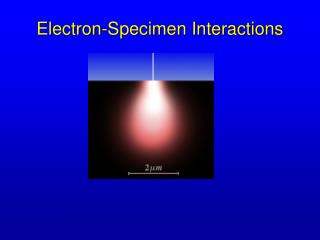
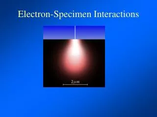
Interaction volume… • Scattering processes operate concurrently • Elastic scattering • Beam electrons deviate from original path – diffuse through solid • Inelastic scattering • Reduce energy of primary beam electrons until absorbed by solid • Limits total electron range • Interaction volume = • Region over which beam electrons interact with the target solid • Deposits energy • Produces radiation • Three major variables • Atomic # • Beam energy • Tilt angle Estimate either experimentally or by Monte Carlo simulations
Monte Carlo simulations Can study interaction volumes in any target Detailed history of electron trajectory Calculated in step-wise manner Length of step? Mean free path of electrons between scattering events Choice of event type and angle Random numbers Game of chance
Casino (2002) Alexandre Real Couture McGill University Dominique Drouin Raynald Gouvin Pierre Hovington Paula Horny Hendrix Demers Win X-Ray (2007) Addscomplete simulation of the X-ray spectrum and the charging effect for insulating specimens McGill University group and E. Lifshin SS MT 95(David Joy – Modified by Kimio Kanda) Run and analyze effects of differing… Atomic Number Beam Energy Tilt angle Note changes in … Electron range Shape of volume BSE efficiency
Labradorite (Z = 11) Monazite (Z = 38) 15 kV 10 kV 1 mm Electron trajectory modeling - Casino
Labradorite (Z = 11) Monazite (Z = 38) 1mm 1mm 5mm 5mm 10 kV 15 kV 20 kV 25 kV 30 kV 10 kV 15 kV 25 kV 30 kV 20 kV =Backscattered
75% 50% 25% 10% 5% Energy contours Electron energy Labradorite [.3-.5 (NaAlSi3O8) – .7-.5 (CaAl2Si2O8), Z = 11] 100% 1% 15 kV
Labradorite (Z = 11) Monazite (Z = 38) 1mm 1mm 5mm 5mm 20 kV 25 kV 30 kV 10 kV 15 kV 15 kV 10 kV 20 kV 25 kV 30 kV = Backscattered Electron energy 100% 1%
10 kV 50% 1 mm 5 kV 25% (~ Ca K ionization energy) 10% 1 kV (~ Na K ionization energy) 5% 5% 10% 25% 50% 75% 100% Labradorite [.3-.5 (NaAlSi3O8) – .7-.5 (CaAl2Si2O8), Z = 11] 15 kV