Download
1 / 22
230 likes | 414 Views
Generalised linear models. Generalised linear model Exponential family Example: logistic model - Binomial distribution Deviances R commands for generalised linear models. Shortcomings of general linear model.

E N D
Generalised linear models • Generalised linear model • Exponential family • Example: logistic model - Binomial distribution • Deviances • R commands for generalised linear models
Shortcomings of general linear model There are three main assumptions behind linear models: 1) Model is linear on parameter; 2) errors are additive; 3) errors have 0 mean, equal variances and they are uncorrelated. For designing hypothesis testing, assumption that errors have normal distribution is also used. These simple assumptions help to solve sufficiently large class of problems and to build models for large class of processes. What happens if these assumptions are not valid? If the fist assumption is not valid then we can use non-linear models. Violation of the second assumption may be problematic then mixed model approach (one of the next lectures) may help to deal with this problem. If the third assumption is violated (more precisely if assumptions that errors have equal variance) then there is an approach to deal with them. That is generalised linear model and it works for large class of distributions. If errors do not have 0 mean then we may subtract mean value of errors and add the mean value as part of the model. If errors are not uncorrelated then either multivariate distributions or mixed model approach may be helpful.
Shortcomings of general linear model: example log(area+1) survived died 1.35 13 0 1.60 19 0 1.75 67 2 1.85 45 5 1.95 71 8 2.05 50 20 2.15 35 31 2.25 7 49 2.35 1 12 Data on survival rate from third degree burns. The number of individuals is 435. If we plot fraction of died vs log(area+1) we see that dependence looks like sigmoidal. We can immediately make several observations: Dependence is not linear and fraction of survived must be between 0 and 1. If we would use simple linear model then for very large values of log(area+1) we would get more than 1 and for very small values we would get negative values. Moreover linear model would have systematic deviations from responses as it can be seen from the figure. Variances are also not uniform over the range of observations. Of course we could try non-linear models and use iterative procedures to fit the model parameters. But are there natural ways of finding a model for this type of cases? In other words: Is there natural generalisation of linear models? Linear model is wrong
Shortcomings of general linear model: Binomials distribution Diagnostics do not look right. Errors (fitted vs residuals) seem to be dependent on fitted values and correlation between fitted and observed values is not very good.
Shortcomings of general linear model: Binomials distribution If the distribution of the observations is binomial then we know that variance is dependent on mean. So the at least one of the conditions, the third condition is violated. In general in these cases one can build a modification of the least-squares equations by addition of weight and solve them: It is weighted least-squares equation. This approach is used in many cases. Usually W is a diagonal of weights. The main problem with this approach is how to design weights. Even if we can design weights the problem of linear model with non-sensical prediction remains. It can also be overcome by either transforming observations (we will touch this topic later) or building non-linear models. Fortunately there is an elegant approach to deal with type of problem – generalised linear models.
Generalised linear model Generalised linear model is a way of extending linear models to deal with observations from wide range of distributions. If the distribution of the observations is from the family of generalised exponential family and mean value (or some function of it) of this distribution is linear on the input parameters then generalised linear model can be used. Generalised exponential family has the form: Many known distributions belong to the generalised exponential family (for simplicity we take S()=1). Other members of this family include: gamma, exponential and many others.
Generalised linear model: Exponential family Natural exponential family of distributions has a form: S() is a scale parameter. Without loss of generality we can replace A() by by change of variables. In this case is called canonical parameter Many distributions including normal, binomial, Poisson, exponential distributions belong to this family. Moment generating function is: Then the first moment (mean value) and the second central moment are:
Generalised linear model If the distribution of observations is one of the distributions from the exponential family and some function of the expected value of the observations is a linear function of the parameters then generalised linear model can be used: Function g is called the link function. That is a function that links observations with parameters of interest, or it links predictors with responses. Some of the popular distributions and corresponding link functions include: binomial - logit = ln(p/(1-p)) it is also known as log of odds normal - identity linear models Gamma - inverse Poisson - log log linear models All good statistical packages have implementation of several generalised linear models. To fit using generalised linear model, maximum likelihood technique is used.
Link function and parameters Canonical link function for exponential families are equal to canonical parameter: For example for normal distribution it is identity function: For binomial distribution it is logit function: For Poisson distribution it is
Generalised linear model: maximum likelihood Let us write it with canonical parameter with natural link function Here we assumed that the form of the distributions for different observations are the same but parameters are different. It is a non-linear optimisation problem. This type of problems are usually solved iteratively. One of the techniques of iterative optimisation is Gauss-Newton. Unfortunately closed form relations (unbiasedness of mean, equations for covariance estimator) that hold for linear models cannot be used here. All properties of generalised linear model are true only asymptotically.
Poisson distribution: log-linear model If the distribution of the observations is Poisson then log-linear model could be used. Recall that Poisson distribution is from exponential family and the function A of the mean value is logarithm. It can be handled using generalised linear model. When log-linear model is appropriate: When outcomes are frequencies (expressed as integers) then log-linear model is appropriate. When we fit log-linear model then we can find estimated mean using exponential function:
Binomial distribution: logistic model If the distribution of the results of experiment is binomial, i.e. outcomes are 0 or 1 (success or failure) then logistic model can be used. Recall that a natural parameter that is a function of the mean value and has a form: This function has a special name – logit. It has several advantages: If logit(p) has been estimated then we can find p and it will always be between 0 and 1. If probability of success is larger than failure then this function is positive, otherwise it is negative. Changing places of success and failure changes only the sign of this function. As it can be seen this function is log of odds. If logit(p) is linear then we can find p: For logistic model either grouped variables (fraction of successes) or individual items (every individual have success (1) or failure (0)) can be used. Ratio of the probability of success to the probability of failure is also called odds.
Example Let us try logistic model for the example of fraction of deaths from third degree burns. Fit of the model to the observations and prediction power of the model is much better. As a result for death probability we will have: After logistic regression it is also possible to calculate log of odds of survival. As it can be seen log of odds is a linear function of the parameters (log of odds is considered to be better than odds themselves because it is symmetric)
GLM diagnostics and fitted vs observed Now diagnostics (predicted vs residuals and fitted vs observed) looks much better. Errors seem to be more or less uniform and predicted and fitted values correlate much better.
Tests for generalised linear models Tests applied for linear model are not easily extended to generalised linear models. In linear models such statistics as t.test, F.test are in common use. Validity of these tests are justified if the distributions of observations are normal. One of the general statistical tests that is used in many different applications is likelihood ratio test. Let us remind us what is likelihood ratio test?
Likelihood ratio test Let us assume that we have a sample of size n (x=(x1,,,,xn)) and we want to estimate a parameter vector =(1,2). Both 1 and 2can also be vectors. We want to test null-hypothesis against alternative one: Let us assume that likelihood function is L(x| ). Then likelihood ratio test works as follows: 1) Maximise the likelihood function under null-hypothesis (I.e. fix parameter(s) 1 equal to 10 , find the value of likelihood at the maximum, 2)maximise the likelihood under alternative hypothesis (I.e. unconditional maximisation), find the value of the likelihood at the maximum, then find the ratio: w is the likelihood ratio statistic. Tests carried out using this statistic are called likelihood ratio tests. In this case it is clear that: If the value of w is small then null-hypothesis is rejected. If g(w) is the the density of the distribution for w then critical region can be calculated using:
Deviances In linear model, we maximise the likelihood with full model and under the null hypothesis. The ratio of the values of the likelihood function under two hypotheses (null and alternative) is related to F-distribution. Interpretation is that how much variance would increase if we would remove part of the model (null hypothesis). In logisitc and log-linear models, again likelihood function is maximised under the null and alternative hypotheses. Then logarithm (it is called deviance) of ratio of the values of the likelihood under these two hypotheses asymptotically has chi-squared distribution: That is the difference between maximum achievable log-likelihood and the value of likelihood at the estimated parameters That is the reason why in log-linear and logistic regressions it is usual to talk about deviances and chi-squared statistics instead of variances and F-statistics. Analysis based on log-linear and logistic models (in general for generalised linear models) is usually called analyisis of deviances. Reason for this is that chi-squared is related to deviation of the fitted model and observations. Another test is based on Pearson’s chi-squared test. It approaches asymptotically to chi-squared with n-p (n is the number of observations and p is the number parameters) degrees of freedom.
Example Let us take the data esoph from R. data(esoph) That is a data set “from a case-control study of (o)esophageal cancer in Ile-et-Vilaine, France” attach(esoph) model1 = glm(cbind(ncases,ncontrols) ~ agegp + tobgp * alcgp,data = esoph, family = binomial()) summary(model1) gives all sort of information about each parameters. They meant to show significance of each estimated parameter. It also gives information about deviances. Null deviance corresponds to the fit with one parameter and residual deviance with all parameters.
R commands for log-linear model log-linear model can be analysed using generalised linear model. Once the responses, independent variables, the formula and family have been decided then we can use: result <- glm(data~formula,family=‘poisson’) It will give us fitted model. Then we can use plot(result) summary(result) Interpretation of the results is similar to that for linear model. Degrees of freedom is defined similarly. Only difference is that instead of sum of squares deviances are used.
R commands for logistic regression Similar to log-linear model: Decide what are the data, the factors and what formula should be used. Then use generalised linear model to fit. result <- glm(data~formula,family=‘binomial’) then analyse using anova(result,test=“Chisq”) summary(result) plot(result) Both AIC and cross-validation can be applied for model selection in generalised linear models. Commands for model selection using AIC is step(glmobject) And for cross-validation is cv.glm(glmobject)
Bootstrap There are different ways of applying bootstrap for these cases: • Sample the original observation with design matrix • Sample the residuals and add them to the fitted values (for each member of family and each link function it should be done differently) • Use estimated parameters and do parametric sampling. • fit the model (using glm and family of distributions) • For each cell in the design matrix find the parameters of the distribution • Sample using the distribution with this parameter • Fit the model again and save coefficients (or any other statistics of interest) • Repeat 3 and 4 B times • Build distributions and other properties
References • McCullagh P. and Nelder, J. A. (1989) Generalized Linear Models. London: Chapman and Hall. • Myers, RM, Montgomery, DC and Vining GG. Generalized linear models: with application in Engineering and the Sciences • McCullagh CP, Searle, (2001) Generalized, linear and mixed models