Download
1 / 28
300 likes | 337 Views
Explore habitat selection models and population dynamics within different environments to understand how populations selectively inhabit spaces, influencing overall species distribution and abundance.

E N D
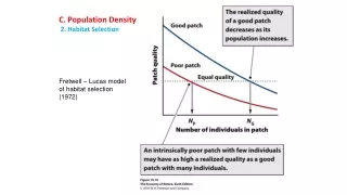
C. Population Density 2. Habitat Selection Fretwell – Lucas model of habitat selection (1972)
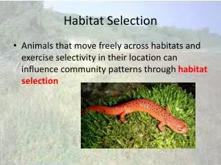
C. Population Density 3. Maintenance of Marginal Populations Why don’t these adapt to local conditions?
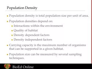
D. Modeling the Spatial Structure of Populations 1. Metapopulation Model Subpopulation inhabit separate patches of the same habitat type in a “matrix” of inhospitable habitat.. - immigration causes recolonization of habitats in which population went extinct. So, rates of immigration and local extinction are critical to predicting long-term viability of population.
D. Modeling the Spatial Structure of Populations 2. Source-Sink Model Subpopulations inhabit patches of different habitat quality, so there are ‘source’ populations with surplus populations that disperse to populations in lower quality patches (‘sinks’).
D. Modeling the Spatial Structure of Populations 3. Landscape Model Subpopulations inhabit patches of different habitat quality, so there are ‘source’ populations with surplus populations that disperse to populations in lower quality patches (‘sinks’). However, the quality of the patches is ALSO affected by the surrounding matrix… alternative resources, predators, etc. And, the rate of migration between patches is also affected by the matrix between patches… with some areas acting as favorable ‘corridors’
E. Macroecology “Top-down” approach – what can the large scale patterns in abundance, density, and diversity tell us?
E. Macroecology 1. Some General Patterns - Species with high density in center of range often have large ranges
E. Macroecology 1. Some General Patterns - Species of large organisms have smaller populations
E. Macroecology 1. Some General Patterns - And of course, food limits size/density relationships
E. Macroecology 1. Some General Patterns - energy equivalency rule: pop’s of biologically similar organisms consume the same amount of energy/unit area, but process it in different ways depending on body size….LATER
E. Macroecology 2. The shapes of ranges - Abundant species have ranges running E-W; rare species have N-S ranges
E. Macroecology 2. The shapes of ranges So, if a species has an E-W range, it will probably cross many habitats; signifying that the species is an abundant generalist.
E. Macroecology 2. The shapes of ranges So, if a species has an E-W range, it will probably cross many habitats; signifying that the species is an abundant generalist. If a species has a N-S distribution, it may be a rare specialist limited to one habitat zone.
E. Macroecology 2. The shapes of ranges So, if a species has an E-W range, it will probably cross many habitats; signifying that the species is an abundant generalist. If a species has a N-S distribution, it may be a rare specialist limited to one habitat zone. An independent test would be to make predictions about Europe.
E. Macroecology 2. The shapes of ranges An independent test would be to make predictions about Europe.
E. Macroecology 2. The shapes of ranges An independent test would be to make predictions about Europe. Abundant species run N-S, and rare species run E-W, as predicted by topography and the generalist-specialist argument.
Population Ecology • Attributes of Populations • Distributions • III. Population Growth – change in size through time • Calculating Growth Rates • 1. Discrete Growth With discrete growth, N(t+1) = N(t)λ Or, Nt = Noλt
Population Ecology • Attributes of Populations • Distributions • III. Population Growth – change in size through time • Calculating Growth Rates • 1. Discrete Growth With discrete growth, N(t+1) = N(t)λ Or, Nt = Noλt Suppose a population doubles each generation (λ = 2), from an initial population of 6. N(t+1) = N(t)λ= 12 = (6) 2 N(t+2) = N(t+1)λ= 24 = (12) 2 After 5 generations, N5 = Noλ5 = 192 = (6) 25 = 6 x 32
Population Ecology • Attributes of Populations • Distributions • III. Population Growth – change in size through time • Calculating Growth Rates • 2. Exponential Growth – continuous reproduction With discrete growth: N(t+1) = N(t)λ or Nt = Noλt Continuous growth: Nt = Noert Where r = intrinsic rate of growth (per capita and instantaneous) and e = base of natural logs (2.72) So, λ = er
Population Ecology • Attributes of Populations • Distributions • III. Population Growth – change in size through time • Calculating Growth Rates • 2. Exponential Growth – continuous reproduction Continuous growth: Nt = Noert Where r = intrinsic rate of growth (per capita and instantaneous) and e = base of natural logs (2.72) So, λ = er And r = Ln (λ) A population will double each time interval if: r = 0.693
So, λ = er • If λ is between zero and 1, then r < 0 and the population will decline. • If λ = 1, then r = 0 and the population size will not change. • If λ >1, then r > 0 and the population will increase. • Population Ecology • Attributes of Populations • Distributions • III. Population Growth – change in size through time • Calculating Growth Rates • 3. Equivalency
The rate of population growth is measured as: The derivative of the growth equation: Nt = Noert dN/dt = rNo • Population Ecology • Attributes of Populations • Distributions • III. Population Growth – change in size through time • Calculating Growth Rates • 3. Equivalency
Population Ecology • Attributes of Populations • Distributions • III. Population Growth – change in size through time • Calculating Growth Rates • 4. Doubling Times Using Nt = Noert If r and N0 are known, then we can calculate 2Nt and solve for t Suppose a population has r = 0.693, and a current population of 32. And we want to know how many time intervals (years) it will take for the population to double to 64.
Population Ecology • Attributes of Populations • Distributions • III. Population Growth – change in size through time • Calculating Growth Rates • 4. Doubling Times Nt = Noert 64 = 32e(0.693)t Divide both sides by 32: 64/32 = 2 = e(0.693)t Take natural logs of both sides: Ln(2) = (0.693)t 0.693/0.693 = 1 = t. Check! Using Nt = Noert If r and N0 are known, then we can calculate 2Nt and solve for t Suppose a population has r = 0.693, and a current population of 32. And we want to know how many time intervals (years) it will take for the population to double to 64.
Population Ecology • Attributes of Populations • Distributions • III. Population Growth – change in size through time • Calculating Growth Rates • 5. Human Population Using dN/dt = Nor We can calculate r from any two population sizes: Human population 2014: 7.24 billion Human population 2015: 7.32 billion So, dN/dt = 80 million = (7.24 billion)r 0.08 x 10⁹/7.24 x 109 = 0.0110 = 1.10% increase
Population Ecology • Attributes of Populations • Distributions • III. Population Growth – change in size through time • Calculating Growth Rates • 5. Human Population Assuming this r, how long to reach 10 billion? Nt = Noert 10 billion = (7.32 billion) e(0.011)t 10/7.32 = 1.366 = e(0.0166)t Ln(1.366) = 0.011t 0.312/0.011 = 28.36 = t So, roughly 29 years from 2015 = 2044. Using dN/dt = Nor We can calculate r from any two population sizes: Human population 2014: 7.24 billion Human population 2015: 7.32 billion So, dN/dt = 80 million = (7.24 billion)r 0.12 x 10⁹/7.24 x 109 = 0.011 = 1.1% increase
Population Ecology • Attributes of Populations • Distributions • III. Population Growth – change in size through time • Calculating Growth Rates • 5. Human Population • Thankfully, r is declining