Download
1 / 14
140 likes | 473 Views
Lecture 5 – Transport pr operties of gases Ch 24 pages 625-627 Summar y of lecture 4 We can use Maxwell-Boltzmann distribution to calculate the average values for any property that depends on speed, e.g. Summar y of lecture 4

E N D
Lecture 5 – Transport properties of gases Ch 24 pages 625-627
Summary of lecture 4 • We can use Maxwell-Boltzmann distribution to calculate the average values for any property that depends on speed, e.g.
Summary of lecture 4 • We have then used simple arguments on mechanical motion in a gas composed of identical particles to provide expression for properties that describe the random motions of molecules in a gas • We have introduced the diffusion coefficient as a measure of the distance traveled over time (on average) by a particle undergoing diffusion:
Summary of lecture 4 • Thediffusion coefficient for a one-component gas is: • The diffusion coefficient depends on molecular properties such as size and molecular weight • Today we will formally describe the motion of particles in a gas (random walk problem), then introduce the continuum description of this same motion (diffusion) • We want to relate microscopic properties of the molecules we study (size, shape, solvation, etc.) to measurable experimental parameters of diffusive motion
Microscopic View of Diffusion: Random Walk • The motion of individual molecules in gases or fluids allows us to explore microscopic aspects of diffusion • Let us for consider the motions a solute molecule (e.g. DNA or protein under electrophoresis or centrifugation) surrounded by solvent molecules with which it collides. If the trajectory (pathway) of an individual solvent molecule is traced out, it appears to be a random walk, much like the zig-zag motion of the molecules in an ideal gas we described in the last lecture
Microscopic View of Diffusion: Random Walk • The average displacement <r> of the solute molecule after time t is indicated by the dark bold line in the figure
Microscopic View of Diffusion: Random Walk • Other molecules will be displaced in other directions. For every solute molecule displaced x as shown, there will be another solute molecule with a displacement in the opposite direction –x. The displacements will all average to zero, that is • However, the mean-squared displacement is non-zero. The random-walk description allows us to calculate this averages
Microscopic View of Diffusion: Random Walk • Many processes in nature including the motion of a drunk man on the way home, Brownian particles, motions of gas molecules, and the average shape of a linear polymer, can be treated as “random walk” problems • The question to be addressed is: what is the average distance between the beginning and end of a path of N random steps of length l?
Microscopic View of Diffusion: Random Walk • In the texbook and lecture notes, you will find formal derivations for these averages • After the rather complex mathematical manipulations reported there, you will find the two strikingly simple results • First, the net forward displacement is 0, while the mean square displacement and mean square displacements are:
Microscopic View of Diffusion: Random Walk • These expressions are stating that, after N steps, one is (on average) away from where it started. The mean displacement is always 0, because the probability of moving back or forward is the same. For any random walk, the root mean square displacement is the microscopic unit displacement times the square root of the total number of hops. This is a fundamental property of random walk.
Random Walk and Diffusion Let us consider now the random diffusion of a molecule in a gas; each molecule will move in a straight line until it encounters another molecule with which it collides The length of each step the random walk is the mean free path l, The rate at which the step will be interrupted is determined by the collisional rate, the number of collision per second For the random diffusion of molecules in a gas, the mean square displacement of each molecule is:
Random Walk and Diffusion Thus, although the average speed of a particle in a gas is very high (>100 m/s) it takes a very long time for molecules to diffuse in a gas because the root mean square displacement is inversely proportional to the rate at which molecules collide
Random Walk and Diffusion The probability W of a random walk of N steps having taken m steps forward is: Once we know the probability, we know everything (in a statistical sense). For example, the average number of steps forward is: The mean of the square of the number of steps forward is:
Random Walk and Diffusion We have expressed the probability in terms of a number displacement, but it is useful to do so in terms of the net distance displacement x=lm where l is the unit displacement (the length of each step taken). Through a simple substitution: Suppose the number of hops or steps per unit time is N’. Then the number of hops N=N’t. Therefore we can also express this probability in terms of frequency of steps and time: