Download
1 / 17
170 likes | 295 Views
EE599-020 Audio Signals and Systems. Formant Estimation Kevin D. Donohue Electrical and Computer Engineering University of Kentucky. Speech Generation.

E N D
EE599-020Audio Signals and Systems Formant Estimation Kevin D. DonohueElectrical and Computer EngineeringUniversity of Kentucky
Speech Generation Speech can be divided into fundamental building blocks of sounds referred to as phonemes. All sounds results from turbulence through obstructed air flow The vocal cords create quasi-periodic obstructions of air flow as a sound source at the base of the vocal tract. Phonemes associated with the vocal cord are referred to as voiced speech. Single shot turbulence from obstructed air flow through the vocal tract is primarily generated by the teeth, tongue and lips. Phonemes associated with with non-periodic obstructed air flow are referred to as unvoiced speech. Taken from http://www.kt.tu-cottbus.de/speech-analysis/
Voiced Speech Quasi-Periodic Pulsed Air Vocal Tract Filter Vocal Radiator Air Burst or Continuous flow Unvoiced Speech Speech Production Models The general speech model: Sources can be modeled as quasi periodic impulse trains or random sequences of impulse. Vocal tract filter can be modeled as an all-pole filter related to the tract resonances. The radiator can be modeled as a simple gain with spatial direction (possibly some filtering)
Vocal Tract Resonances First 3 resonances of tube with 1 closed end Vocal tract length corresponds to signal wavelength (). It can be obtained from resonant frequencies (f ) estimated from recorded speech soundsand the speed of sound (c), using equation: 1/4 Wavelength 3/4 Wavelength 5/4 Wavelength Image adapted from:hyperphysics.phy-astr.gsu.edu
Vocal Tract Resonances The resonances of the vocal tract are called formants and can be estimated from peaks of the spectrum where the effects of pitch have been smoothed out (i.e. spectral envelope).
Low Order AR Modeling If the voiced speech is characterized by an all pole model with low order (i.e. about 10), then the frequencies of the poles correspond to the resonances of the vocal tract. This filter effectively predicts the value of the next sample from previous samples. Therefore it is call a linear prediction filter (LPC).
Example Create an “augh” sound (as the “a” in about or “u” in hum) and use the (linear prediction coefficient) LPC command to model this sound being generated from a quasi-periodic sequence of impulses exciting an all pole filter. The LPC command finds a vector of filter coefficients such that prediction error is minimized: Predict x(n) from previous samples: Compute prediction error sequence with: Use Z-transforms to find transfer function of filter that recovers x(n) from the LPCs and error sequence e(n). Identify the components related to source, vocal tract, and radiator.
LPC Derivation Derive an algorithm to compute LPC coefficients from a stream of data that minimizes the mean squared prediction error. Let be the sequence of data points and be the mth order LPC coefficients, and be the prediction estimate. The mean squared error for the prediction is given by:
LPC Computation Put prediction equations in matrix form: Each row of is a prediction of samples in rows of
LPC Computation The mean squared error can be expressed as: If derivative is taken with respect to a and set equal to 0, the result is:
Autocorrelation and LPC Define the autocorrelation of a sequence as: Note that the LPC coefficients are computed from the autocorrelation coefficients: Autocorrelation Matrix
Script for Analysis [y,fs] = wavread('aaaaa.wav'); % Read in wave file [cb,ca] = butter(5,2*100/fs,'high'); % Filter to remove LF recording noise yf = filtfilt(cb,ca,y); [a,er] = lpc(yf,10); % Compute LPC coefficent with model order 10 predy = filter(a,1,yf); % Compute prediction error with all zero filter (FIR) figure(1) ; plot(predy); title('Prediction error'); xlabel('Samples'); ylabel('Amplitude') recon = filter(1,a,predy); % Compute reconstructed signal from error and all-pole filter (IIR) figure(2) % Plot reconstructed signal plot(recon,'b') hold on % Plot with original delayed by a unit so it does not entirely overlap the perfectly reconstructed signal plot(yf(2:end),'r') hold off % By examining a the error sequence, generate a simple impulse sequence to simulate its period (about 103 sample period) g = []; for k=1:150 g = [g, 1, zeros(1,103)]; end % Run simulated error sequence through all pole filter sim = filter(1,a,g); soundsc([(sim')/std(sim); yf/std(yf)],fs) % Play sounds compare simulated with real
Script for Analysis % Plot pole zero diagram figure(3) r = (roots(a)) w = [0:.001:2*pi]; plot(real(r),imag(r),'xr',real(exp(j*w)),imag(exp(j*w)),'b'); title('Pole diagram of vocal tract filter') xlabel('Real'); ylabel('Imaginary') % Find resonant frequencies corresponding to poles froots = (fs/2)*angle(r)/pi; nf = find(froots > 0 & froots < fs/2); % Find those corresponding to complex conjugate poles figure(4) % Examine average specturm with formant frequencies [pd,f] = pwelch(yf, hamming(2*1024),256,4*1024,fs); dbspec = 20*log10(pd); mxp = max(dbspec); % Find max and min points for graphing verticle lines mnp = min(dbspec); plot(f,dbspec,'b') % Plot PSD hold on % Over lines on plot where formant frequencies were estimated from LPCs for k=1:length(nf) plot([froots(nf(k)), froots(nf(k))], [mnp(1), mxp(1)], 'k--') end hold off title('PSD plot with formant frequencies (Black broken lines)'); xlabel('Hertz'); ylabel('dB')
LPC Analysis Result Pole Frequencies of LPC model from vocal tract shape Frequency periodicities from harmonics of Pitch frequency
… z-1 z-1 z-1 z-1 + Vocal Tract Filter Implementations Direct form 1 for all pole model:
z-1 z-1 z-1 z-1 + + + + + + + + + Vocal Tract Filter Implementations Direct form 1, second order sections: … z-1 z-1
+ + + + + z-1 z-1 Vocal Tract Filter Implementations Lattice implementation are popular because of error and stability properties. The filter is implement in modular stages with coefficients directly related to stability criterion and tube resonances of the vocal tract : z-1