A Prototype Finite Difference Model
A Prototype Finite Difference Model. A Prototype Model. We will introduce a finite difference model that will serve to demonstrate what a computational scientist needs to do to take advantage of Distributed Memory computers using MPI


A Prototype Finite Difference Model
E N D
Presentation Transcript
A Prototype Model • We will introduce a finite difference model that will serve to demonstrate what a computational scientist needs to do to take advantage of Distributed Memory computers using MPI • The model we are using is a two dimensional solution to a model problem for Ocean Circulation, the Stommel Model
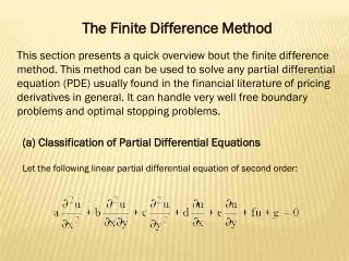
The Stommel Problem • Wind-driven circulation in a homogeneous rectangular ocean under the influence of surface winds, linearized bottom friction, flat bottom and Coriolis force. • Solution: intense crowding of streamlines towards the western boundary caused by the variation of the Coriolis parameter with latitude
Governing Equations Model Constants 2 2 ¶ y ¶ y ¶ y ( ) f b g + + = 2 2 x ¶ x y ¶ ¶ y p f s i n ( ) = - a 2L y L L 2 0 0 0 K m = = x y ( 6 ) - 3 1 0 g = * ( 1 1 ) - 2 . 2 5 1 0 b = * ( 9 ) - 1 0 a =
Domain Discretization D e f i n e a g r i d c o n s i s t i n g o f p o i n t s ( x , y ) g i v e n b y i j x i x , i 0 , 1 , . . . . . . . , n x + 1 = D = i y j y , j 0 , 1 , . . . . . . . , n y + 1 = D = j x L ( n x 1 ) D = + x y L ( n y 1 ) D = + y
Domain Discretization Seek to find an approximate solution ( x , y ) a t p o i n t s ( x , y ) : y i i j j ( x , y ) y » y i , j i j
Centered Finite Difference Scheme for the Derivative Operators
Five-point Stencil Approximationfor the Discrete Stommel Model i, j+1 interior grid points: i=1,nx; j=1,ny boundary points: (i,0) & (i,ny+1) ; i=1,nx (0,j) & (nx+1,j) ; j=1,ny i, j i-1, j i+1, j i, j-1
Jacobi Iteration Start with an initial guess for do i = 1, nx; j = 1, ny end do Copy Repeat the process
Overview • Model written in Fortran 90 • Uses many new features of F90 • Free format • Modules instead of commons • Module with kind precision facility • Interfaces • Allocatable arrays • Array syntax
Free Format • Statements can begin in any column • ! Starts a comment • To continue a line use a “&” on the line to be continued
Modules instead of commons • Modules have a name and can be used in place of named commons • Modules are defined outside of other subroutines • To “include” the variables from a module in a routine you “use” it • The main routine stommel and subroutine jacobi share the variables in module “constants” module constants real dx,dy,a1,a2,a3,a4,a5,a6 end module … program stommel use constants … end program subroutine jacobi use constants … end subroutine jacobi
Kind precision facility Instead of declaring variables real*8 x,y We use real(b8) x,y Where b8 is a constant defined withina module module numz integer,parameter::b8=selected_real_kind(14) end module program stommel use numz real(b8) x,y x=1.0_b8 ...
Kind precision facility Why? Legality Portability Reproducibility Modifiability real*8 x,y is not legal syntax in Fortran 90 Declaring variables “double precision” will give us 16 byte reals on some machines integer,parameter::b8=selected_real_kind(14) real(b8) x,y x=1.0_b8 Gives us a real with at least 14 digits precision on all platforms Declare all variables using this syntax we can change precision by changing a single line
Allocatable arrays • We can declare arrays to be allocatable • Allows dynamic memory allocation • Define the size of arrays at run time real(b8),allocatable::psi(:,:) ! our calculation grid real(b8),allocatable::new_psi(:,:) ! temp storage for the grid ! allocate the grid to size nx * ny plus the boundary cells allocate(psi(0:nx+1,0:ny+1)) allocate(new_psi(0:nx+1,0:ny+1))
Interfaces • Similar to C prototypes • Can be part of the routines or put in a module • Provides information to the compiler for optimization • Allows type checking module face interface bc subroutine bc (psi,i1,i2,j1,j2) use numz real(b8),dimension(i1:i2,j1:j2):: psi integer,intent(in):: i1,i2,j1,j2 end subroutine end interface end module program stommel use face ...
Array Syntax Allows assignments of arrays without do loops ! allocate the grid to size nx * ny plus the boundary cells allocate(psi(0:nx+1,0:ny+1)) allocate(new_psi(0:nx+1,0:ny+1)) ! set initial guess for the value of the grid psi=1.0_b8 ! copy from temp to main grid psi(i1:i2,j1:j2)=new_psi(i1:i2,j1:j2)
Program Outline (1) • Module NUMZ - defines the basic real type as 8 bytes • Module INPUT - contains the inputs • nx,ny (Number of cells in the grid) • lx,ly (Physical size of the grid) • alpha,beta,gamma (Input calculation constants) • steps (Number of Jacobi iterations) • Module Constants - contains the invariants of the calculation
Program Outline (2) • Module face - contains the interfaces for the subroutines • bc - boundary conditions • do_jacobi - Jacobi iterations • force - right hand side of the differential equation • Write_grid - writes the grid
Program Outline (3) • Main Program • Get the input • Allocate the grid to size nx * ny plus the boundary cells • Calculate the constants for the calculations • Set initial guess for the value of the grid • Set boundary conditions • Do the Jacobi iterations • Write out the final grid
C version considerations • To simulate the F90 numerical precision facility we: • #define FLT double • And use FLT as our real data type throughout the rest of the program • We desire flexibility in defining our arrays and matrices • Arbitrary starting indices • Contiguous blocks of memory for 2d arrays • Use routines based on Numerical Recipes in C
Vector allocation routine FLT *vector(INT nl, INT nh) { /* creates a vector with bounds vector[nl:nh]] */ FLT *v; /* allocate the space */ v=(FLT *)malloc((unsigned) (nh-nl+1)*sizeof(FLT)); if (!v) { printf("allocation failure in vector()\n"); exit(1); } /* return a value offset by nl */ return v-nl; }
Matrix allocation routine FLT **matrix(INT nrl,INT nrh,INT ncl,INT nch) /* creates a matrix with bounds matrix[nrl:nrh][ncl:nch] */ /* modified from the book version to return contiguous space */ { INT i; FLT **m; /* allocate an array of pointers */ m=(FLT **) malloc((unsigned) (nrh-nrl+1)*sizeof(FLT*)); if (!m){ printf("allocation failure 1 in matrix()\n"); exit(1);} m -= nrl; /* offset the array of pointers by nrl */ for(i=nrl;i<=nrh;i++) { if(i == nrl){ /* allocate a contiguous block of memroy*/ m[i]=(FLT *) malloc((unsigned) (nrh-nrl+1)*(nch-ncl+1)*sizeof(FLT)); if (!m[i]){ printf("allocation failure 2 in matrix()\n");exit(1); } m[i] -= ncl; /* first pointer points to beginning of the block */ } else { m[i]=m[i-1]+(nch-ncl+1); /* rest of pointers are offset by stride */ } } return m; }