Download

1 / 35
380 likes | 799 Views
Frequency-Domain Analysis and stability determination. frequency-response studies. In practice, the performance of a control system is more realistically measured by its time-domain characteristics.

E N D
frequency-response studies • In practice, the performance of a control system is more realistically measured by its time-domain characteristics. • The reason is that the performance of most control systems is judged based on the time due to certain test signals. • But, there are some systems which has input signal of sinusoidal function. • The frequency domain is also more convenient for measurements of system sensitivity to noise and parameter variations.
the steady-state output of the system, y(t), will be a sinusoid with the same frequency ω but possibly with different amplitude and phase; that is, • then the Laplace transforms of the input and the output are related through • For sinusoidal steady-state analysis, we replace s by jω, and the last equation becomes • By writing the function Y(jω) as
with similar definitions for M(jω) and R(jω), leads to the magnitude relation between the input and the output: and the phase relation: • Thus, for the input and output signals described on the above eqns, respectively, the amplitude of the output sinusoid is • and the phase of the output is
Frequency Response of Closed-Loop Systems • the closed-loop transfer function is • Under the sinusoidal steady state, s = jω, • The magnitude of M(jω) is • and the phase of M(jω) is
Frequency-Domain Specifications • Specifications such as the maximum overshoot, damping ratio, and the like used in the time domain can no longer be used directly in the frequency domain. The following frequency-domain specifications are often used in practice. • Resonant Peak (Mr) • The resonant peak Mr is the maximum value of • Normally, a large Mr corresponds to a large maximum overshoot of the step response. For most control systems, it is generally accepted in practice that the desirable value of Mr should be between 1.1 and 1.5. Resonant Frequency (ωr) • The resonant frequency ωr, is the frequency at which the peak resonance Mr occurs.
Bandwidth BW • The bandwidth BW is the frequency at which drops to 70.7% of, down from, its zero frequency value. • In general, the bandwidth of a control system gives indication on the transient-response properties in the time domain. A large bandwidth corresponds to a faster rise time, since higher-frequency signals are more easily passed through the system. • Resonant Peak and Resonant Frequency • For the prototype second-order system, the resonant peak Mr, the resonant frequency ωr and the bandwidth BW are all uniquely related to the damping ratio ξ, and the natural undamped frequency ωn of the system. • Consider the closed-loop transfer function of the prototype second-order system
At sinusoidal steady state, s = jω, • by letting u = ω/ωn, • The magnitude and phase of M(jω) are and The resonant frequency is determined by
Therefore the value of U and ω, and Because frequency is a real quantity, is meaningful only for 2ξ< 1, or ξ < 0.707. The value of Mr for u and simplifying, we get It is important to note that, for the prototype second-order system, Mr is a function of damping ratio ξ only, and is a function of both ξ and ωn.
Bandwidth • In accordance with the definition of bandwidth, we set the value of M(ju) to . • the bandwidth of the prototype second-order system is determined • Therefore
NYQUIST STABILITY CRITERION: • Nyquist criterion is a semigraphical method that determines the stability of a closed System by investigating the properties of the frequency-domain plot, the Nyquist plot, of the loop transfer function G(s)H(s), or L{s). • The Nyquist plot of L(s) is a plot of L (jω) in the polar coordinates of lm[L(jω)] versus Re[L(jω)] as to varies from 0 to ∞. • Let us consider that the closed-loop transfer function • where G(s)H(s) can assume the following form
Because the characteristic equation is obtained by setting the denominator polynomial of M(s) to zero, • In general, for a system with multiple number of loops, the denominator of M(s) can be written as • Loop transfer function zeros: zeros of L(s) • Loop transfer function poles: poles of L(s) • Closed-loop transfer function poles: zeros of 1 + L(s) = roots of the characteristic equation • poles of 1 + L(s) = poles of L(s). • Stability Conditions • Closed-Loop Stability: A system is said to be closed-loop stable, or simply stable, if the poles of the closed-loop transfer function or the zeros of 1 + L(s) are all in the left-half S-plane. Exceptions to the above definitions are systems with poles or zeros intentionally placed at s = 0.
Suppose that a continuous closed path Гs is arbitrarily chosen in the s-plane, as shown in Fig, If Гs does not go through any poles of ∆(s), then the trajectory Г∆ mapped by ∆(s) into the ∆(s) -plane is also a closed one, as shown in Fig. below. The direction of traverse of Г∆ can be either CW or CCW, that is, in the same direction or the opposite direction as that of Гs, depending on the function ∆(s).
“Let ∆(s) be a single-valued function that has a finite number of poles in the s-plane. Suppose that an arbitrary closed path Гs is chosen in the s-plane so that the path does not go through any one of the poles or zeros of ∆(s); the corresponding Г∆ locus mapped in the ∆(s)-plane will encircle the origin as many times as the difference between the number of zeros and poles of ∆(s) that are encircled by the s-plane locus Гs.” In equation form, the principle of the argument is stated as N = Z-P, where N --number of encirclements of the origin made by the ∆(s)-plane locus Г∆. Z --number of zeros of ∆(s) encircled by the S-plane locus Гs in the S-plane. P--number of poles of ∆(s) encircled by the S -plane locus Гs in the S-plane.
Let us consider the function ∆(s) is of the form • The function ∆(s) can be written as
Because the poles of ∆(s) contribute to a negative phase, and zeros contribute to a positive phase, the value of N depends only on the difference between Z and P. For the case illustrated Z = 1 and P = 0. Thus, N = Z - P = 1 • Which means that the ∆(s)-plane locus Г∆ should encircle the origin once in the same direction as that of the s-plane locus Гs • If there are N more zeros than poles of ∆(s) , which are encircled by the s-plane locus Гs, in a prescribed direction, the ∆(s) -plane locus will encircle the origin N times in the same direction as that of Гs. • Conversely, if N more poles than zeros are encircled by Гs in a given direction, N will be negative, and the ∆(s)-plane locus must encircle the origin N times in the opposite direction to that of Гs.
Nyquist Criterion and the L(s) or the G(s)H(s) Plot • In principle, once the Nyquist path is specified, the stability of a closed-loop system can be determined by plotting the ∆(s)= 1 +L(s) locus when S takes on values along the Nyquist path. • Because the function L(s) is generally known, it would be simpler to construct the L(s) plot that corresponds to the Nyquist path, and the same conclusion on the stability of the closed-loop system can be obtained by observing the behavior of the L(s) plot with respect to the (-1, j0) point in the L(s)-plane.
Nyquistcriterion to the stability problem involves the following steps. • The Nyquist path Гs is defined in the s-plane, • The L(s) plot corresponding to the Nyquist path is constructed in the L(s)-plane. • The value of N, the number of encirclement of the (-1, j0) point made by the L(s) plot, is observed. • The Nyquist criterion follows from N = Z-P That is, “for a closed-loop system to be stable, the L{s)plot must encircle the (-l, j0) point as many times as the number of poles of L(s) that are in the right-half s-plane, and the encirclement, if any, must be made in the clockwise direction (if Гs is defined in the CCW sense)
Example: Consider that a single-loop feedback control system has the loop transfer function • The stability of the closed-loop system can be conducted by investigating whether the Nyquist plot of L(jω)/K for ω = 0 to ∞ encloses the (-1, j0) point. 1. Substitute s = jω in L(s). 2. Substituting ω = 0 in the last equation, we get the zero-frequency property of L(j ω) 3. Substituting ω = ∞ , the property of the Nyquist plot at infinite frequency is established.
4. To find the intersect(s) of the Nyquist plot with the real axis, if any, we rationalize L(jω)/K 5. To find the possible intersects on the real axis, we set the imaginary part of L(jω)/K to zero. The result is • The solutions of the last equation are ω = ∞ , which is known to be a solution at L(jω)/K = 0, and • Because ω is positive, the correct answer is ω= ±20 rad/sec. Substituting this frequency
Thus, we see that, if K is less than 240, the intersect of the L(jω) locus on the real axis would be to the right of the critical point (-1, j0); the latter is not enclosed, and the system is stable. If K = 240, the Nyquist plot of L(jω) would intersect the real axis at the -1 point, and the system would be marginally stable.
Gain Margin (GM) Gain Margin (GM) is one of the most frequently used criteria for measuring relative stability of control systems. • In the frequency domain, gain margin is used to indicate the closeness of the intersection of the negative real axis made by the Nyquist plot of L( jω) to the (-1, j0) point. • Phase Crossover: A phase-crossover on the L(jω) plot is a point at which the plot intersects the negative real axis. • Phase-Crossover Frequency: The phase-crossover frequency ωp is the frequency at the phase crossover, or where
L(jω) at ω= ωp is designated as |L(jωp)|. Then, the gain margin of the closed-loop system that has L(s) as its loop transfer function is defined as
we can draw the following conclusions about the gain margin • The L(jω) plot does not intersect the negative real axis (no finite nonzero phase crossover). • The L(jω) plot intersects the negative real axis between (phase crossover lies between) 0 and the 1 point. • The L(jω) plot passes through (phase crossover is at) the (-1 , j0) point. • The L(jω) plot encloses (phase crossover is to the left of) the (-1, j0) point.
Gain margin is the amount of gain in decibels (dB) that can be added to the loop closed-loop system becomes before the closed-loop unstable. • When the Nyquist plot does not intersect the negative real axis at any finite nonzero frequency, the gain margin is infinite in dB; this means that, theoretically, the value of the loop gain can be increased to infinity before instability occurs.
When the Nyquist plot of L(jω) passes through the (-1, j0) point, the gain margin is 0 dB, which implies that the loop gain can no longer be increased, as the system is at the margin of instability. • When the phase-crossover is to the left of the (-1, j0) point, the phase margin is negative in dB, and the loop gain must be reduced by the gain margin to achieve stability.
Phase Margin (PM) • The gain margin is only a one-dimensional representation of the relative stability of a closed-loop system. • As the name implies, gain margin indicates system stability with respect to the variation in loop gain only. • To include the effect of phase shift on stability, we introduce the phase margin,
Gain Crossover: The gain crossover is a point on the L(jω) plot at which the magnitude of L(jω) is equal to 1. Gain-Crossover Frequency: The gain-crossover frequency, ωg, is the frequency of L(jω) at the gain crossover. Or where |L(jωg)| = 1 The definition of phase margin is stated as: Phase margin (PM) is defined as the angle in degrees through which the L(jω) plot must be rotated about the origin so that the gain crossover passes through the (-1, j0).
The analytical expression of the phase margin, • Example • As an illustrative example on gain and phase margins, consider that the loop transfer function of a control system is • The following results are obtained from the Nyquist plot: • Gain crossover ωg =6.22rad/sec • Phase crossover ωp = 15.88 rad/sec • The magnitude of L(jωp) is 0.182. Thus, the gain margin is obtained from • The phase of L(jωg) is 211.72°. Thus, the phase margin is obtained from
STABILITY ANALYSIS WITH THE BODE PLOT • The Bode plot of a transfer function is a very useful graphical tool for the analysis and design of linear control systems in the frequency domain. • Advantages of the Bode Plot 1. In the absence of a computer, a Bode diagram can be sketched by approximating the magnitude and phase with straight line segments. 2. Gain crossover, phase crossover, gain margin, and phase margin are more easily determined on the Bode plot than from the Nyquist plot. 3. For design purposes, the effects of adding controllers and their parameters are more easily visualized on the Bode plot than on the Nyquist plot.
The following observations can be made on system stability with respect to the properties of the Bode plot: 1. The gain margin is positive and the system is stable if the magnitude of L(jω) at the phase crossover is negative in dB. That is, the gain margin is measured below the 0-dB-axis. If the gain margin is measured above the 0-dB-axis, the gain margin is negative, and the system is unstable. 2. The phase margin is positive and the system is stable if the phase of L{jω) is greater than -180° at the gain crossover. That is, the phase margin is measured above the -180°-axis. If the phase margin is measured below the -180°-axis, the phase margin is negative, and the system is unstable.
Example • Consider the loop transfer function given • The Bode plot is shown below
The gain crossover is the point where the magnitude curve intersects the 0-dB axis. The gain crossover frequency ωg is 6.22 rad/sec. The phase margin is measured at the gain crossover. The phase margin is measured from the -180°-axis and is 31.72°. Because the phase margin is measured above the -180°-axis, the phase margin is positive, and the system is stable. • The phase crossover is the point where the phase curve intersects the -180°-axis. The phase crossover frequency is ωp = 15.88 rad/sec. The gain margin is measured at the phase crossover and is 14.8 dB. Because the gain margin is measured below the 0-dB-axis, the gain margin is positive, and the system is stable.