Enhanced Depth Estimation and Focus Recovery Study
400 likes | 424 Views
Explore methods for depth estimation and focus recovery in digital images involving Fourier and geometric optics, camera lens structure, and aberration solutions. Investigate binocular and stereo vision techniques for depth perception.

Enhanced Depth Estimation and Focus Recovery Study
E N D
Presentation Transcript
Depth Estimation and Focus Recovery(景深估計與聚焦重建) Speaker: Yu-Che Lin ( 林于哲) Adviser : Prof. Jian-Jiun Ding (丁建均 教授) Digital Image and Signal Processing Laboratory (DISP) MD-531
Outlines • Motivations • Overview on previous works • Structure of camera lens / Geometric optics • Introduction to Fourier optics • Blurring function / Equal-focal assumption • Binocular / Stereo vision • Vergence • Monocular • Depth from focus • Estimator of degree on focus / Sum of Laplacian • Interpolation • Depth from defocus • Arbitrary changing camera parameters with large variation • Trace amount on changing camera parameters Digital Image and Signal Processing Laboratory (DISP) MD-531
Linear canonical transform (LCT) upon the optical system • Linear canonical transform (LCT) • Approximation on the optical system by LCTs • Focus recovery: common method, alternative method • The common method • Alternative method: one point focus recovery • Simulation on simple pattern • Conclusions • References Digital Image and Signal Processing Laboratory (DISP) MD-531
Motivations • Depth is an important information for robot and the 3D reconstruction. • Image depth recovery is a long-term subject for other applications such as robot vision and the restorations. • Most of depth recovery methods based on simply camera focus and defocus. • Focus recovery can help users to understand more details for the original defocus images. Digital Image and Signal Processing Laboratory (DISP) MD-531
Overview on previous works Digital Image and Signal Processing Laboratory (DISP) MD-531
Structure of camera lens (1) cited on : http://en.wikipedia.org/wiki/Concave_lens#Types_of_lenses • Physical lens. • Structure of camera lens against the aberration (像差) • Two of aberrations : Chromatic (色像) , Spherical aberration. Higher wavelength, lower refractive index convex concave cited on : http://en.wikipedia.org/wiki/Concave_lens#Types_of_lenses cited on : http://en.wikipedia.org/wiki/Index_of_refraction Digital Image and Signal Processing Laboratory (DISP) MD-531
Common solutions for aberrations: “Asperical” lens and complementary lenses (Groups). One shot always has multiple lenses. Geometric on imaging. F : focal length u: object dist. v: imaging dist. D: lens diameter R: blurring radius s: dis. between lens and screen (CCD) Structure of camera lens (2) Complementary convex and concave lenses cited on : http://www.schneideroptics.com/info/photography.htm Digital Image and Signal Processing Laboratory (DISP) MD-531
F L2 L1 Structure of camera lens (3) • Combination by lenses of the real camera. • The effective focal length : • Due to the above effective value, we can now just ignore the complicated combinations. Digital Image and Signal Processing Laboratory (DISP) MD-531
. . . . . . Introduction to Fourier optics (1) • Aperture effect. When the wave incident through an aperture, the observed field is the combination: • The unperturbed incident wave by geometric optics. • A diffractive wave originating from the rim of the aperture. • Diffraction. • Fresnel principle ( near-field diffraction ) • Fraunhofer principle ( far-field diffraction ) strict on field distance, Digital Image and Signal Processing Laboratory (DISP) MD-531
Introduction to Fourier optics (2) • The Huygens-Fresnel transform. • Considering a square wave : Digital Image and Signal Processing Laboratory (DISP) MD-531
x1 x0 r01 P1(x1,y1) P0(x0,y0) y1 y0 Introduction to Fourier optics (3) • The field intensity through the circular aperture (ex: camera aperture ) by unit amplitude plane wave under Fraunhofer diffraction theory is actually a sinc function . • The structure inside the camera shot should more like a near-field condition , so the intensity pattern acts more like a Gaussian function. Digital Image and Signal Processing Laboratory (DISP) MD-531
Blurring radius: R<0 Blurring radius: R>0 v F F D/2 s u screen 2R : R>0 F F screen D/2 s u 2R : R<0 Biconvex v Blurring function / Equal-focal assumption (1) Digital Image and Signal Processing Laboratory (DISP) MD-531
Blurring function / Equal-focal assumption (2) • Due to geometric optics, the intensity inside the blur circle should be constant. • Considering of aberration and diffraction and so on, we easily assume a blurring function: • : diffusion parameter • Diffusion parameter is related to blur radius: • Derived from triangularity in geometric optics • For easy computation, we always assume that foreground has equal-diffusion, background has equal-diffusion and so on • However, this equal-focal assumption will be a problem K: calibrated by each specific camera Digital Image and Signal Processing Laboratory (DISP) MD-531
Binocular / Stereo vision Digital Image and Signal Processing Laboratory (DISP) MD-531
Vergence • Vergence movement : • is some kind of slow eye movement that two eyes move in different directions. • Disadvantage : • Correspondence problem ( trouble ). Digital Image and Signal Processing Laboratory (DISP) MD-531
Depth from focus Digital Image and Signal Processing Laboratory (DISP) MD-531
Estimator of degree on focus / Sum of Laplacian • Actively taking pictures at different observer distance or object distance . • Estimator of degree on focus. • we need an operator to abstract how “ focused ” the region is • Since the blur model is a low pass filter, the estimator can be a Laplacian • Such operator point to a measurement on a single pixel influence, a sum of Laplacian operator is needed: Digital Image and Signal Processing Laboratory (DISP) MD-531
NP Measured curve Focus measure Nk Ideal condition Nk-1 Nk+1 [SML] dp dk-1 dk dk+1 displacement Interpolation (1) • We use Gaussian interpolation to form a set of approximations. • We have dp that is the camera displacement performing perfect focused : • , Digital Image and Signal Processing Laboratory (DISP) MD-531
Interpolation (2) • The depth solution dp from above Gaussian : Digital Image and Signal Processing Laboratory (DISP) MD-531
Depth from defocus Digital Image and Signal Processing Laboratory (DISP) MD-531
Arbitrary changing camera parameters with large variation • Two diffusion parameters are considering. • Intuitively, we can get two pictures by changing one of camera parameters and solve the triangularity problem. On the spatial domain or frequency domain. Replace to solve u i : equal focal subimage Digital Image and Signal Processing Laboratory (DISP) MD-531
Trace amount on changing camera parameters (1) • More accurate by changing camera parameters with trace amount. • We use the power spectral density : • Utilizing the fact that differential on the Gaussian function is still a Gaussian. Digital Image and Signal Processing Laboratory (DISP) MD-531
Trace amount on changing camera parameters (2) • We have no idea on diffusion parameters, but we can replace it by camera parameters by differential factor. Digital Image and Signal Processing Laboratory (DISP) MD-531
Linear canonical transform (LCT) upon the optical system Digital Image and Signal Processing Laboratory (DISP) MD-531
Linear canonical transform (LCT) (1) • Linear canonical transform (LCT) : • The LCT gives a scalable kernel to describe wave propagation such as the fractional Fourier transform and the Fresnel transform and etc. • Definition (normalize as four parameters). Digital Image and Signal Processing Laboratory (DISP) MD-531
Linear canonical transform (LCT) (2) • Through a brief derivation, we can see that a combination of the LCTs is still a LCT. • The reason for the parameters mapping is for its convenience coordinates transformation on the time-frequency distribution. • Some important properties connected by the LCT : • Scaling, phase delay (chirp multiplication), modulation, chirp convolution and the fractional Fourier transform. Digital Image and Signal Processing Laboratory (DISP) MD-531
Linear canonical transform (LCT) (3) • Sinc value in the frequency domain of a rectangle signal in the time domain. Its parameters of LCT (A,B,C,D) = (0,1,-1,0) : the Fourier transform. Digital Image and Signal Processing Laboratory (DISP) MD-531
z s Uo Ul Ul’ Ui Approximation on the optical system by LCTs • We now consider a simple and common optical system. • The effective LCT parameters : Phase delay (chirp multiplication) Free space diffraction (chirp convolution) Digital Image and Signal Processing Laboratory (DISP) MD-531
Focus recovery: common method, alternative method Digital Image and Signal Processing Laboratory (DISP) MD-531
K1 g1 R1 f K2 g2 R2 The common method (1) • The most common focus recovery method : • Based on the assumption that a simply constructed image scene has two layers, foreground and background. • Two input images, one focus on foreground ( f1 ) and the other focus on background ( f2 ). Using adjustable values R1 and R2 to generate images. • Where ( i= 1, 2, a, b ) indicates point spread functions, note that a and b are adjusted parameters • -- Design filters K1 and K2 !! Digital Image and Signal Processing Laboratory (DISP) MD-531
The common method (2) • The matrix form. • Considering the existence of the inverse matrix (singular or nonsingular). Digital Image and Signal Processing Laboratory (DISP) MD-531
The common method (3) • Filters result. Digital Image and Signal Processing Laboratory (DISP) MD-531
These blurred areas are too large for the HVS and result in two blurring areas. Larger Aperture Position of object F 。。。 。。。 。。。 thin lens sensor Alternative method :one point focus recovery (1) • Depth of field (DOF). • The ideal case (larger aperture). Digital Image and Signal Processing Laboratory (DISP) MD-531
Smaller Aperture Position of object 。 。 。 F sensor thin lens These blurred areas are too small for the HVS and results in an effective focused plane. Effective “depth of field” interval Alternative method :one point focus recovery (2) • The effective focused interval (smaller aperture). Digital Image and Signal Processing Laboratory (DISP) MD-531
Alternative method :one point focus recovery (3) • Approximation by LCTs. • Paraxial approximation (phase delay). • The original Fresnel transform : Digital Image and Signal Processing Laboratory (DISP) MD-531
Defocused image pair SML measurement Maximum value searching focal point Depth measurement of a point Using the specific depth to retrieve imaging distance Small aperture construction Linear canonical transform based on constructed optical system Full focused image Alternative method :one point focus recovery (4) • Flow chart for the alternative method : one point focus recovery. Digital Image and Signal Processing Laboratory (DISP) MD-531
a b c d Simulation on simple pattern • Considering the Gaussian point light source. • For simplicity, we assumes the parameters : • (a) – the input Gaussian pattern. • (b) – LCT for s = 27 mm. • (c) – LCT for s = 30 mm. • (d) – Inverse LCT for s = 27 mm. Digital Image and Signal Processing Laboratory (DISP) MD-531
Conclusions • Most of the literature discussed on the depth or the depth recovery fall in the equal focal problems (DFD, DFF) or the correspondent problems (stereo vision). • Relying on the LCTs by the paraxial approximation system can avoid such problems. • Using LCTs is more like a deblurring procedure. Such action can keep the original realities of the images from disturbance. Digital Image and Signal Processing Laboratory (DISP) MD-531
References • Y. Xiong and S. A. Shafer, “Depth from focusing and defocusing,” IEEE Conference on Computer Vision and Pattern Recognition, pp. 68-73, 1993. • M. Subbarao, “Parallel depth recovery by changing camera parameters,” Second International Conference on Computer Vision, 1988, pp. 68-73, 1988. • K. S. Pradeep and A. N. Rajagopalan, “Improving shape from focus using defocus information,” 18th International Conference on Pattern Recognition, 2006, vol. 1, p.p. 731-734, Sept. 2006. • M. Asif and A. S. Malik, T. S. Choi “3D shape recovery from image defocus using wavelet analysis,” IEEE International Conference on Image Processing, 2005, vol. 1, pp. 11-14, Sept. 2005. • K. Nayar and Y. Nakagawa, “Shape from focus,” IEEE Transactions on Pattern Analysis and Machine Intelligence, vol. 16, issue 8, pp. 824-831, Aug, 1994. Digital Image and Signal Processing Laboratory (DISP) MD-531
Y. Y. Schechner and N. Kiryati, “Depth from defocus vs. stereo: how different really are they?,” in ICPR 1998, vol. 2, pp. 1784-1786, Aug. 1998. • M. Haldun Ozaktas, Zeev Zalevsky and M. Alper Kutay, “The fractional Fourier transform with applications in optics and signal processing,”JOHN WILEY & SONS, LTD, New York, 2001. • A. Kubota and K. Aizawa, “Inverse filters for reconstruction of arbitrarily focused images from two differently focused images,”IEEE Conferences on Image Processing 2000, vol.1, pp.101-104, Sept. 2000. • A. P. Pentland, “A new sense for depth of field”, IEEE Transaction on Pattern Analysis and Machine Intelligence, vol. 9, no. 4, pp. 523-531, 1987. • M. Hansen and G. Sommer, “Active depth estimation with gaze and vergence control using gabor filters,”, Proceedings of the 13th International Conference on Pattern Recognition 1996, vol. 1, pp. 287-291, Aug. 1996. Digital Image and Signal Processing Laboratory (DISP) MD-531