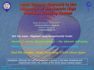
Least Squares Approach to the Alignment of the Generic High Precision Tracking System

1. Least Squares Approach to the Alignment of the Generic High Precision Tracking System PHYSTAT’05 Oxford 14/09/05 Pawel Brückman de Renstromp.bruckman@physics.ox.ac.ukStephen HaywoodS.Haywood@rl.ac.uk Set the scene: Alignment using reconstructed tracks Decent 2 versus unbiased physics – the inherent deficiency Possible extensions to the formalism – extra handles Real life example: simple tests using ATLAS silicon layout Disclaimer: Although the method presented is generic it has been developed and implemented within the context of the ATLAS silicon tracking system.

2. Acknowledgements • We would like to thank the ATLAS Inner Detector Alignment Group for helpful discussions. In particular, we acknowledge valuable discussions and cross-checks provided by Adlene Hicheur and thank him for his collaboration. • The datasets used have been generated using ATLAS software, for which we thank the ATLAS Software Team. • This work is an extension of ideas used by ALEPH: ALEPH-97-116, A. Bonissent et al. • The approach to the alignment of ATLAS silicon system has been documented in ATL-COM-INDET-2005-04.

3. Barrel SCT Forward SCT Forward PIXels Barrel PIXels ATLAS Silicon Tracking System 3 translations & 3 rotations of each module In total we have to deal with 34,992 DoF’s!

4. Si Sensors Hybrid with ASICs ASICs ~70mm ~140mm Si Sensor TPG+BeO Baseboard An example of the BarrelSCT module • PIXel detectors provide real 2-D readout. • Pixels are of size 50400 m resulting in 14115 m resolution. • SCT modules are double-sided strip detectors with 1-D readout per side. • Sensitive strips have pitch of 80 m giving 23 m resolution. • Stereo angle of 40 mrad gives 580 m resolution in the other direction. • The entire tracker is equipped with the binary readout.

5. Global2 fit – the idea

6. The inherent dilemma • Assure decent fit of all tracks – easy  A “simple” global 2 minimisation using both track and alignment parameters should be sufficient. • Provide an unbiased physics output – highly nontrivial!  This means we want the fitted track parameters to be unbiased. There is a lot of global distortions of the detector geometry which result in biases. These correspond to low frequency modes, so-called “weak modes”, of the solution of the above 2. It will become clearer when discussing a real life example. The two are coupled but only weakly. The first should asymptotically converge to the latter provided there are no systematic effects in the reconstruction. In real life systematics always occur and statistical sample is ‘rarely’ infinite.

7. “Weak modes” - examples “clocking” R (VTX constraint) radial distortions (various) “telescope” z~R • dependent sagitta • XabRcR2 • dependent sagitta “Global twist” • Rcot() • We need extra handles in order to tackle these. • The natural candidates are: • Requirement of a common vertex for a group of tracks (VTX constraint), • Constraints on track parameters or vertex position, • External constraints on alignment parameters. global sagitta R …

8. track Intrinsic measurement error + MCS hit residual Key relation! Direct Least-Squares solution to the alignment problem The method consists of minimizing the giant 2resulting from a simultaneous fit of all particle trajectories and alignment parameters: Let us consequently use the linear expansion (we assume all second order derivatives are negligible). The track fit is solved by: while the alignment parameters are given by:

9. The Millepede Aposteriori we realised that our baseline formalism is equivalent to the one of V. Blobel and C. Kleinwort. They arrive at the same solution using purely matrix manipulation method:  VERY reassuring! Is strictly the same formula! V.Blobel, C.Kleinwort, “A new method for the high-precision alignment of track detectors” Proceedings of the Conference on: Advanced Statistical Techniques in Particle Physics University of Durham, UK March 18th-22nd, 2002 http://www.ippp.dur.ac.uk/Workshops/02/statistics/proceedings.shtml

10. The “Real Life” Example • Test setup consists of a cone of the barrel PIX + SCT corresponding to approx. 0<<1. • The geometry contains 1030 silicon modules i.e. 6180 DoF’s. • Data sample consists of 500,000 muon tracks with transverse momenta 2 < pT< 20 GeV. • Disclamer: Track statistics are small and in the following we will discus solution properties rather than try to demonstrate the ultimate achievable precision.

11. Example “lowest modes” in PIX+SCT as reconstructed by the 2algorithm Global Freedom have been ignored (only one Z slice shown) singular modes • The above “weak modes” contribute to the lowest part of the eigen-spectrum. Consequently they dominate the overall error on the alignment parameters. • More importantly, these deformations lead directly to biases on physics (systematic effects).

12. PIX TEST 1 Realignment of the “ideal” detector using the baseline algorithm. Grey are the nominal positions, blue corrected ones. Radial distortion to PIXel detector corresponding to “weak modes” is clearly visible Displacements exaggerated by a factor 100 !!!

13. TEST 2 • Re-alignment of the distorted detector. PIXel modules were collectively shifted by: • (X=200m, Y=100m, Z=400m) • in the ATLAS global frame. • (a difficult distortion – much worse than random displacements!) • Tracks were refitted to the modified hit positions. • The alignment algorithm was run using the refitted tracks • In order to improve clarity and reduce underlying statistical fluctuations the displacements depicted on the left are the differences between corrections resulting from this test and the ones obtained from realignment of the undistorted detector (Test 1). Displacements exaggerated by a factor 100 !!!

14. Jacobian (mode itself) X (m) Y (m) Z (m) -198 5 -1055 -45029 -199 4 -1024 -44527 -200 3 -1013 -44025 -2 3 03 -2215 -2 2 02 -1610 -1 1 01 -25 0 0 00 00 Fixed to 0 A quantitative insight TEST 2 (cont) In order to have more quantitative insight we do projection on rigid cylinders: The technique may prove very useful as a day-0 solution or a genuine method to reduce number of DoF’s. E.g.: think of addressing “weak modes” separately without having to worry about large matrix inversion. Simple and powerful tool on its own! Re-alignment of the distorted detector. PIXel detector was collectively shifted by: (X=200m, Y=100m, Z=400m) The resulting corrections to the rigid cylinders are: The fit settles on a minor “telescope” mode.

15. New key relations! Direct Least-Squares solution to the alignment problem (2) Fitting a common vertex for a group of tracks We follow the same principle but now we have Individual track parameters are reduced to while tracks from the same vertex share the same set of three parameters describing the common vertex position. where Using the new form of the full derivative we obtain solution for the alignment parameters: were we have defined:

16. PIX TEST 3 Realignment of the “ideal” detector using the algorithm with the common Vertex fit. Distortions to the PIXel detector are significantly reduced Displacements exaggerated by a factor 100 !!!

17. A quantitative comparison Errors on PIX positions reduced as expected Sensitivity to low modes improved!

18. Direct Least-Squares solution to the alignment problem (3) Adding constraints on track parameters Here we show the simplest case of a direct constraint on track parameters and without the vertex fit. We start from the redefined 2 and the respective solution for track parameters: J The solution is given by the modified formula where the redefined form of the track weight matrix J is used throughout: Similarly, one can write out solution for the most general case including VTX fit and constraints on all formal parameters.

19. TEST 4 Realignment of the “ideal” detector imposing constraints on certain track parameters: cot() -= 0.001, (cot()=0.0001 Q/pT -= 0.01 GeV-1, (Q/pT)=0.001 Resulting distortions to the detectror are as expected (sagitta+”telescope”) “telescope”: cot() shift z~R Sagitta: Q/pT shift ~R

20. TEST 4 (cont.) Realignment of the “ideal” detector imposing constraints on certain track parameters: cot() -= 0.001, (cot()=0.0001 Q/pT -= 0.01 GeV-1, (Q/pT)=0.001 Tracks (sample of 500) were refitted to the new geometry. Plotted are the track-by-track differences between the initial and refitted parameters of the track. (only the relevant two shown)

21. Constraint on mass of a resonance Idea of the constraints on track parameters can be extended to a constraint on the mass of a known resonance (e.g. Z+-, J/ +) As a result (in full analogy to the basic constraint on track parameters) the track parameter weight matrix gets modified and there is an extra term added to the big vector of the final system of equations:

22. Constraint on the mass of a resonance TEST 5 The idea has been tested in a very naïve way using the multi-muon event sample. Tracks with pT>5 GeV were combined into pseudo-resonances if the resulting mass was 5 GeV or larger. The measured mass was used for the M value in each case.  was et to 0.1 GeV. Results are encouraging but the method clearly deserves proper validation using true Z and J/ samples. improvement

23. End-cap SCT 842 simultaneous length measurements in SCT! Barrel SCT End-cap SCT 165 165 80+(3x[80+16])+(2x72)=512 END FLANGES B3 B4,5,6 Using external constraints on the geometry Frequency Scanning Interferometry: • Single FSIGridLineInterferometer has a precision below1m! • Entire Grid shape can be determined to better than10m in 3D. • FSI provides quasi real-time response to time dependent deformations.

24. Using external constraints on the geometry Extra terms added to the weight matrix and the big vector of the final system of equations:

25. Using external constraints on the geometry TEST 6 Mode#4 was constrained to amplitude A=1 and =0.01. After diagonalisation of the matrix M this mode was found to have: A=0.987, =0.0099 which is consistent with the imposed constraint. All other modes acquired the same amplitudes as in the unconstrained case. The genuine mode #4 used Difference to the unconstraint case

26. Settled on a “telescope” with A=0.255 “telescope” eradicated A=0.000 Using external constraints on the geometry TEST 7 Mode#10 (“telescope”) was constrained to amplitude A=0 and =0.001. After diagonalisation of the matrix M this mode was found to have: A=0.00007, =0.0010 which is consistent with the imposed constraint. All other modes acquired the same amplitudes as in the unconstrained case. The genuine unconstrained solution Difference to the unconstraint case

27. Summary • The minimisation of the global 2 is an optimal method which uses the information in complete and rigorous way. • Due to complexity of the tracking and limits to the processing time linear expansion in track and alignment parameters is the most natural choice. • The problem has an inherent deficiency – low frequency modes of the solution can bias the physics output. • Generic handles helping to “strengthen” the solution have been proposed. • The presented formalism comprising vertex fit and constraints of all formal parameters is well established and has been implemented in the ATLAS software. • More detailed checks (in particular of the numerical stability of the solution) using large sample of simulated physics events are still to come. • The implementation has been designed for ATLAS but could, with some extra effort, be converted into a general purpose package.