Download
1 / 77
770 likes | 910 Views
Linear Algebra in a Computational Setting Alan Kaylor Cline. LASA December 3, 2013. How long does it take for this code to run?. After examining the code you believe that the running time depends entirely upon some input parameter n and …. a good model for the running time is

E N D
Linear Algebrain a Computational SettingAlan Kaylor Cline LASA December 3, 2013
After examining the code you believe that the running time depends entirely upon some input parameter nand … a good model for the running time is Time(n) = a + b·log2(n) + c·n + d·n·log2(n) where a, b, c, and d are constants but currently unknown.
Time(10) = 0.685 ms.Time(100) = 7.247ms.Time(500) = 38.511ms.Time(1000) = 79.134 ms. So you time the code for 4 values of n, namely n = 10, 100, 500, and 1000and you get the times According to the model you then have 4 equations in the 4 unknowns a, b, c, and d: a + b·log2(10) + c·10 + d·10·log2(10) = 0.685 a + b·log2(100) + c·100 + d·100·log2(100) = 7.247 a + b·log2(500) + c·5000 + d·500·log2(500) = 38.511 a + b·log2(1000) + c·1000+ d·1000·log2(1000) = 79.134
a + b·log2(10) + c·10 + d·10·log2(10) = 0.685 a + b·log2(100) + c·100 + d·100·log2(100) = 7.247 a + b·log2(500) + c·5000 + d·500·log2(500) = 38.511 a + b·log2(1000) + c·1000+ d·1000·log2(1000) = 79.134 These equations are linear in the unknownsa, b, c, and d. We solve them and obtain: a = 6.5 b = 10.3 c = 57.1 d = 2.2 So the final model for the running time is Time(n) = 6.5 + 10.3·log2(n) + 57.1·n + 2.2·n·log2(n)
and now we may apply the model Time(n) = 6.5 + 10.3·log2(n) + 57.1·n + 2.2·n·log2(n) for a particular value of n (for example, n = 10,000) to estimate a running time of Time(10,000) = 6.5 + 10.3·log2(10,000) + 57.1· 10,000 + 2.2· 10,000 ·log2(10,000) = 863.47 ms.
So you time the code for 30 values of n, and you get these times {(ni,ti)}
If the model was perfect and there were no errors in the timings then for some values a, b, c, d, and e: a + b·log2(ni) + c·ni + d·ni·log2(ni) +e·ni2 =ti for i =1,…,30
But the model was not perfect and there were error in the timings So we do not expect to get any values a, b, c, d, and e so that: a + b·log2(ni) + c·ni + d·ni·log2(ni) +e·ni2 =ti for i =1,…,30 We will settle for values a, b, c, d, and e so that: a + b·log2(ni) + c·ni + d·ni·log2(ni) +e·ni2 ti for i =1,…,30
Our sense of a+ b·log2(ni) + c·ni + d·ni·log2(ni) +e·ni2 ti for i =1,…,30 Will be to get a, b, c, d, and e so that sum of squares of all of the differences (a+ b·log2(ni) + c·ni + d·ni·log2(ni) +e·ni2 -ti)2 is minimized over all possible choices of a, b, c, d, and e
After solving the least squares system to get the best values of a, b, c, d, and e, we plota + b·log2(n) + c·n + d·n·log2(n) + e·n2
What’s a “good” solutionwhen we don’t have the exact solution?
What’s a “good” solutionwhen we don’t have the exact solution? “Hey. That’s not a question that was discussed in other math classes.”
What’s a “good” solutionwhen we don’t have the exact solution? Consider the two equations:
Consider two approximate solution pairs: and these two equations:
Consider two approximate solution pairs: and these two equations: Which pair of these two is better?
Important fact to consider: The exact solution is: Which pair of these two is better?
Consider two approximate solution pairs: and these two equations: Which pair of these two is better?
Important fact to consider: Recall we are trying to solve: For the first pair, we have: For the second pair, we have: Which pair of these two is better?
Important fact to consider: Which pair of these two is better?
Student: “Is there something funny about that problem?” Professor: “You bet your life. It looks innocent but it is very strange. The problem is knowing when you have a strange case on your hands.” CLINE
Professor: “Geometrically, solving equations is like finding the intersections of lines.” CLINE
When lines have no thickness … here’s the intersection?
… but when lines have thickness … where’s the intersection?
Galveston Island 25.96 miles
Galveston Island 25.96 miles Where’s the intersection?
London Olympics Swimming • http://www.youtube.com/watch?v=fFiV4ymEDfY&feature=related • 1:19
How do you transform this image … into the coordinate system of another image?
and in greater generality, transform 3-dimensional objects
The $25 Billion Eigenvector How does Google do Pagerank?
The $25 Billion Eigenvector How did Google do Pagerank?
The Imaginary Web Surfer: • Starts at any page, • Randomly goes to a page linked from the current page, • Randomly goes to any web page from a dangling page, • … except sometimes (e.g. 15% of the time), goes to a purely random page.
J A A tiny web: who should get the highest rank? B I C H D G F E
The associated stochastic matrix: 0.0150 0.0150 0.0150 0.0150 0.0150 0.0150 0.4400 0.0150 0.0150 0.2983 0.4400 0.0150 0.0150 0.0150 0.0150 0.0150 0.0150 0.0150 0.0150 0.0150 0.0150 0.2983 0.0150 0.0150 0.0150 0.0150 0.0150 0.0150 0.0150 0.0150 0.0150 0.2983 0.8650 0.0150 0.0150 0.0150 0.0150 0.0150 0.0150 0.0150 0.4400 0.0150 0.0150 0.8650 0.0150 0.8650 0.0150 0.0150 0.0150 0.0150 0.0150 0.2983 0.0150 0.0150 0.8650 0.0150 0.0150 0.0150 0.0150 0.0150 0.0150 0.0150 0.0150 0.0150 0.0150 0.0150 0.0150 0.8650 0.0150 0.0150 0.0150 0.0150 0.0150 0.0150 0.0150 0.0150 0.0150 0.0150 0.8650 0.2983 0.0150 0.0150 0.0150 0.0150 0.0150 0.0150 0.0150 0.0150 0.0150 0.2983 0.0150 0.0150 0.0150 0.0150 0.0150 0.0150 0.4400 0.0150 0.0150 0.0150
We seek to find a vector x so thatA x = x One way is to start with some initial x0, and then: for k = 1, 2, 3,… xk = A xk-1 This converges to an x so that A x = x