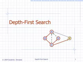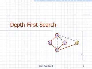
Lecture 15: Depth First Search

1. Lecture 15:Depth First Search Shang-Hua Teng

2. A A B B D F F E E D C C Graphs • G= (V,E) • Directed Graph (digraph) • Degree: in/out • Undirected Graph • Adjacency is symmetric

3. Graph Basics • The size of a graph is the number of its vertices • If two vertices are connected by an edge, they are neighbors • The degree of a node is the number of edges it has • For directed graphs, • The in-degree of a node is the number of in-edges it has • The out-degree of a node is the number of out-edges it has

4. A A B B F A B E E F E C D D D C C F Paths, Cycles path <A,B,F> • Path: • simple: all vertices distinct • Cycle: • Directed Graph: • <v0,v1,...,vk > forms cycle if v0=vk and k>=1 • simple cycle: v1,v2..,vk also distinct • Undirected Graph: • <v0,v1,...,vk > forms (simple) cycle if v0=vk and k>=3 • simple cycle: v1,v2..,vk also distinct simple cycle <E,B,F,E> simple cycle <A,B,C,A>= <B,C,A,B>

5. connected 2 connected components A A A A B B B D D F F F not strongly connected E E E D D C C C C B strongly connected component F E Connectivity • Undirected Graph: connected • every pair of vertices is connected by a path • one connected component • connected components: • equivalence classes under “is reachable from” relation • Directed Graph: strongly connected • every pair of vertices is reachable from each other • one stronglyconnected component • strongly connected components: • equivalence classes under “mutually reachable” relation

6. Subgraphs • A subgraph S of a graph G is a graph such that • The edges of S are a subset of the edges of G • The edges of S are a subset of the edges of G • A spanning subgraph of G is a subgraph that contains all the vertices of G Subgraph Spanning subgraph

7. Trees and Forests • A (free) tree is an undirected graph T such that • T is connected • T has no cycles This definition of tree is different from the one of a rooted tree • A forest is an undirected graph without cycles • The connected components of a forest are trees Tree Forest

8. Spanning Trees and Forests • A spanning tree of a connected graph is a spanning subgraph that is a tree • A spanning tree is not unique unless the graph is a tree • Spanning trees have applications to the design of communication networks • A spanning forest of a graph is a spanning subgraph that is a forest Graph Spanning tree

9. Complete Graphs A graph which has edge between all pair of vertex pair is complete. A complete digraph has edges between any two vertices.

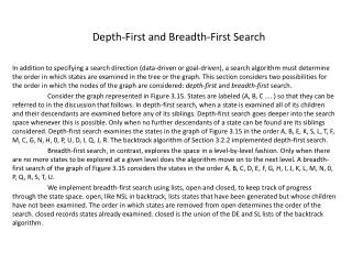
10. Graph Search (traversal) • How do we search a graph? • At a particular vertices, where shall we go next? • Two common framework: the breadth-first search (BFS) and the depth-first search (DFS) • In BFS, one explore a graph level by level away (explore all neighbors first and then move on) • In DFS, go as far as possible along a single path until reach a dead end (a vertex with no edge out or no neighbor unexplored) then backtrack

11. Depth-First Search dfs(g, current) { mark current as visited x = set of nodes adjacent to current for(i gets next in x*) if(i has not been visited yet) dfs(g, i) } * - we will assume that adjacent nodes will be processed in numeric or alphabetical order • The basic idea behind this algorithm is that it traverses the graph using recursion • Go as far as possible until you reach a deadend • Backtrack to the previous path and try the next branch • The algorithm in the book is overly complicated, we will stick with the one on the right • The graph below, started at node a, would be visited in the following order: a, b, c, g, h, i, e, d, f, j d a c b e f g h i j

12. Color Scheme • Vertices initially colored white • Then colored gray when discovered • Then black when finished

13. Time Stamps • Discover time d[u]: when u is first discovered • Finish time f[u]: when backtrack from u • d[u] < f[u]

14. DFS Example sourcevertex

15. DFS Example sourcevertex d f 1 | | | | | | | |

16. DFS Example sourcevertex d f 1 | | | 2 | | | | |

17. DFS Example sourcevertex d f 1 | | | 2 | | 3 | | |

18. DFS Example sourcevertex d f 1 | | | 2 | | 3 | 4 | |

19. DFS Example sourcevertex d f 1 | | | 2 | | 3 | 4 5 | |

20. DFS Example sourcevertex d f 1 | | | 2 | | 3 | 4 5 | 6 |

21. DFS Example sourcevertex d f 1 | 8 | | 2 | 7 | 3 | 4 5 | 6 |

22. DFS Example sourcevertex d f 1 | 8 | | 2 | 7 | 3 | 4 5 | 6 |

23. DFS Example sourcevertex d f 1 | 8 | | 2 | 7 9 | 3 | 4 5 | 6 |

24. DFS Example sourcevertex d f 1 | 8 | | 2 | 7 9 |10 3 | 4 5 | 6 |

25. DFS Example sourcevertex d f 1 | 8 |11 | 2 | 7 9 |10 3 | 4 5 | 6 |

26. DFS Example sourcevertex d f 1 |12 8 |11 | 2 | 7 9 |10 3 | 4 5 | 6 |

27. DFS Example sourcevertex d f 1 |12 8 |11 13| 2 | 7 9 |10 3 | 4 5 | 6 |

28. DFS Example sourcevertex d f 1 |12 8 |11 13| 2 | 7 9 |10 3 | 4 5 | 6 14|

29. DFS Example sourcevertex d f 1 |12 8 |11 13| 2 | 7 9 |10 3 | 4 5 | 6 14|15

30. DFS Example sourcevertex d f 1 |12 8 |11 13|16 2 | 7 9 |10 3 | 4 5 | 6 14|15

31. Pseudocode • DFS(G) • For each v in V, • color[v]=white; p[u]=NIL • time=0; • For each u in V • If (color[u]=white) • DFS-VISIT(u)

32. DFS-VISIT(u) • color[u]=gray; • time = time + 1; d[u] = time; • For each v in Adj(u) do • If (color[v] = white) • p[v] = u; • DFS-VISIT(v); • color[u] = black; • time = time + 1; f[u]= time;

33. Complexity Analysis There is only one DFS-VISIT(u) for each vertex u. Ignoring the recursion calls the complexity is O(deg(u)+1) The recursive call on v is charged to DFS-VISIT(v) Initialization complexity is O(V) Overall complexity is O(V + E)

34. DFS Forest • p[v] = u then (u,v) is an edge • All descendant of u are reachable from u • p defines a spanning forest

35. Parenthesis LemmaRelation between timestamps and ancestry • u is an ancestor of v if and only if [d[u], f[u]] [d[v], f[v]] • u is a descendent of v if and only if [d[u], f[u]][d[v], f[v]] • u and v are not related if and only if [d[u], f[u]] and [d[v], f[v]] are disjoint

36. DFS: Tree (Forest) Edges • DFS introduces an important distinction among edges in the original graph: • Tree edge: encounter new (white) vertex • The tree edges form a spanning forest

37. sourcevertex d f 1 |12 8 |11 13|16 2 | 7 9 |10 3 | 4 5 | 6 14|15 DFS Example Tree edges

38. DFS: Back Edges • DFS introduces an important distinction among edges in the original graph: • Tree edge: encounter new (white) vertex • Back edge: from descendent to ancestor • Encounter a grey vertex (grey to grey)

39. DFS Example sourcevertex d f 1 |12 8 |11 13|16 2 | 7 9 |10 3 | 4 5 | 6 14|15 Tree edges Back edges

40. DFS: Forward Edges • DFS introduces an important distinction among edges in the original graph: • Tree edge: encounter new (white) vertex • Back edge: from descendent to ancestor • Forward edge: from ancestor to descendent • Not a tree edge, though • From grey node to black node

41. DFS Example sourcevertex d f 1 |12 8 |11 13|16 2 | 7 9 |10 3 | 4 5 | 6 14|15 Tree edges Back edges Forward edges

42. DFS: Cross Edges • DFS introduces an important distinction among edges in the original graph: • Tree edge: encounter new (white) vertex • Back edge: from descendent to ancestor • Forward edge: from ancestor to descendent • Cross edge: between a tree or subtrees • From a grey node to a black node

43. DFS Example sourcevertex d f 1 |12 8 |11 13|16 2 | 7 9 |10 3 | 4 5 | 6 14|15 Tree edges Back edges Forward edges Cross edges

44. DFS: Types of edges • DFS introduces an important distinction among edges in the original graph: • Tree edge: encounter new (white) vertex • Back edge: from descendent to ancestor • Forward edge: from ancestor to descendent • Cross edge: between a tree or subtrees • Note: tree & back edges are important; most algorithms don’t distinguish forward & cross

45. DFS: Undirected Graph • Theorem: If G is undirected, a DFS produces only tree and back edges • Proof by contradiction: • Assume there’s a forward edge • But F? edge must actually be a back edge (why?) source F?

46. DFS: Undirected Graph • Theorem: If G is undirected, a DFS produces only tree and back edges • Proof by contradiction: • Assume there’s a cross edge • But C? edge cannot be cross: • must be explored from one of the vertices it connects, becoming a treevertex, before other vertex is explored • So in fact the picture is wrong…bothlower tree edges cannot in fact betree edges source C?

47. DFS Undirected Graph • Theorem: An undirected graph is acyclic iff a DFS yields no back edges • If acyclic, no back edges (because a back edge implies a cycle • If no back edges, acyclic • No back edges implies only tree edges (Why?) • Only tree edges implies we have a tree or a forest • Which by definition is acyclic • Thus, can run DFS to find whether a graph has a cycle

48. Example: DFS of Undirected Graph G=(V,E) Adjacency List: A: B,C,D,F B: A,C,D C: A,B,D,E,F D: A,B,C,G E: C,G F: A,C G: D,E A D B G E C F

49. Example: DFS of Undirected Graph Adjacency List: A: B,C,D,F B: A,C,D C: A,B,D,E,F D: A,B,C,G E: C,G F: A,C G: D,E A D B G E C F

50. Example: DFS of Undirected Graph Adjacency List: A: B,C,D,F B: A,C,D C: A,B,D,E,F D: A,B,C,G E: C,G F: A,C G: D,E A D T B G E C F