Expanded Depth-First Search
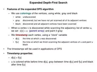
Expanded Depth-First Search. Features of the expanded DFS algorithm We use colorings of the vertices, using white, gray and black white: undiscovered gray: discovered, but we have not yet scanned all of its adjacent vertices black: discovered and all adjacent vertices have been scanned

Expanded Depth-First Search
E N D
Presentation Transcript
Expanded Depth-First Search • Features of the expanded DFS algorithm • We use colorings of the vertices, using white, gray and black • white: undiscovered • gray: discovered, but we have not yet scanned all of its adjacent vertices • black: discovered and all adjacent vertices have been scanned • When a vertex v is discovered while scanning the adjacency list of vertex u, we set [v] = u (parent array) and paint it gray • We timestamp each vertex, using a “clock” variable • d[u] the time at which u was discovered • f[u] the time at which we finish scanning the adjacent vertices of u and paint u black • The timestamps will be used in applications of DFS • Timestamp properties: • d[u] < f[u] • u is colored white before time d[u], gray between time d[u] and f[u] and black after time f[u]
DFS Pseudocode DFS(G) 1 for each vertex u V[G]do color[u] WHITE [u] NIL time 0 5 for each vertex u V[G]do if color[u] = WHITEthen DFS-Visit(u)
DFS Pseudocode DFS-Visit(u) • color[u] GRAY WHITE vertex has just been discovered time time + 1 d[u] time • for each v Adj[u] Explore edge (u,v)do if color[v] = WHITEthen [v] u DFS-Visit(v) • color[u] BLACK • time time + 1 • f[u] time
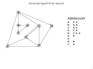
Directed Graph Example • We illustrate the execution of DFS on the digraph below.
Edge Classification • Edges may be classified as follows • Tree edge From a parent to a child in the DFS forest • Back edge From a tree descendant to an ancestor • Forward edge From a tree ancestor to a tree descendant • Cross edge Between vertices in different component tree or between two “cousin” vertices in the same component tree • In our previous example directed graph, the edges are colored according to their classification
Edge Classification in DFS • We may modify the DFS algorithm to classify the edges as they are examined during the search • This method will be unable to distinguish between forward and cross edges • When we look down edge (u,v) while exploring from u, the classification depends on the color of v at that time: • WHITE: (u,v) is a tree edge • GRAY: (u,v) is back edge • BLACK: (u,v) is either a forward edge or a cross edge • TheoremIn a DFS search of an undirected graph every edge is either a tree edge or a back edge.
Running Time DFS(G) 1 for each vertex u V[G]do color[u] WHITE [u] NIL time 0 5 for each vertex u V[G]do if color[u] = WHITEthen DFS-Visit(u) O(|V|) O(|V|) + cost of DFS-Visit Calls
Running Time DFS-Visit(u) • color[u] GRAYtime time + 1 d[u] time • for each v Adj[u] do if color[u] = WHITEthen [v] u DFS-Visit(v) • color[u] BLACK • time time + 1 • f[u] time O(|Adj[v]|) Aggregate Analysis (over all calls)DFS-Visit is called once for each vertex u Total cost: Total Running Time of DFS: O( |V| + |E| )
Properties of DFS • DFS yields valuable information about graph structure • Vertex v is a descendant in the DFS forest of vertex u if and only if v was discovered during the period in which u was colored GRAY Parenthesis Theorem Suppose DFS is run on a directed or undirected graph G = (V,E). Then for any two vertices u,v of G, exactly one of the following three conditions holds: • Intervals [ d[u],f[u] ] and [ d[v],f[v] ] are disjoint and neither u nor v is a descendant of the other in the DFS forest • [ d[u],f[u] ] [ d[v],f[v] ] and u is a descendant of v in the DFS forest • [ d[v],f[v] ] [ d[u],f[u] ] and v is a descendant of u in the DFS forest
Proof of the Parenthesis Theorem • Case 1: d[u] < d[v] • Sub-case 1: d[v] < f[u] Thus v was discovered while u was still colored GRAY v is a descendant of u and f[v] < f[u] and thus the gray interval of v is a subset of the gray interval of u • Sub-case 2: f[u] < d[v]Then the two gray intervals are disjoint since d[u] < f[u] < d[v] < f[v] • Case 2: d[v] < d[u]Same argument as in Case 1 with roles of u and v reversed shows that either the gray interval for u is contained in the gray interval of v or the two gray intervals are disjoint.
Corollary • Corollary to the Parenthesis Theorem Vertex v is a proper descendant of vertex u in the DFS forest for a (directed or undirected) graph G if and only if d[u] < d[v] < f[v] < f[u]
White-Path Theorem White-path Theorem In a DFS forest of a (directed or undirected) graph G = (V,E), vertex v is a descendant of vertex u iff at time d[u], v can be reached from u along a path consisting of only white vertices. Proof If v is a descendant of u in the DFS forest, then all vertices on the path from u to v in the forest (excepting u) must have discovery time later than d[u]. Thus, at time d[u], they are all white, so there is a white path from u to v at time d[u]. We next want to show that if there is a white path from u to v at time d[u], then v is a descendant of u in the DFS forest. Suppose not, and let v be a vertex with the shortest white-path length at time d[u] that is not a descendant of u in the forest and let w be the predecessor of v on a shortest u-v white path at time d[u].
Strongly Connected Components • A strongly connected component of a directed graph G = (V,E) is a subset C of V with the following properties: 1. u,v C, u is reachable from v in G and v is reachable from u in G • If C is a proper subset of another subset D of V, then D does not satisfy property 1 • In short: C is a maximal subset of V having property 1 • Many directed graph algorithms proceed as follows: • decompose the directed graph into its strongly connected components; • run the algorithm separately on each of the strongly connected components • combine the solutions according to the connections between the strongly connected components • Thus we need an efficient algorithm for finding the strongly connected components of directed graphs • Depth-first search is the basis for a (|V| + |E|) method for solving this problem
Strongly Connected Components • We will use the transpose (or reversal) of a directed graph in our algorithm • If G = (V,E) is a digraph, then the transposeGT of G is the digraph with vertex set V and edge set ET = { (v,u) | (u,v) E } • Given an adjacency-list representation of G, the time to create GT is O(|V|+|E|).
Strongly Connected Components Proposition 1 A directed graph and its transpose have exactly the same strongly connected components
Strongly Connected Components Algorithm • The algorithm runs DFS twice • First on G, to compute the finishing times f[u] of each vertex u • Second on GT with vertices considered in order of decreasing f[u] from the run of DFS on G • The DFS trees obtained from the second run of DFS are the strongly connected components Strongly-Connected-Components(G) • call DFS(G) to compute the finishing times f[u] for each vertex u • compute GT • call DFS(GT), but in the main loop of DFS, consider vertices in order of decreasing f[u] as computed in 1 • output the vertices of each tree if the DFS-forest formed in line 3 as a separate strongly connected component
Component Digraph • The component digraph of a directed graph G is the digraph with one vertex vC for each strongly-connected component of G and edges those pairs (vC,vD) such that there is an edge in G from a vertex of C to a vertex of D. • The component digraphs for our previous example is
Component Digraph Lemma Lemma 2 Let C and C be strongly connected components of a digraph G = (V,E), let u, v C, let u,v C, and suppose there is a path from u to u in G. Then there cannot be a path from v to v in G. Corollary The component digraph of a directed graph is a directed acyclic graph
Discovery and Finish Times • In the ensuing discussions, d[u] and f[u] will always refer to the discovery and finishing times during the first call of DFS (on G). Definition If U is a subset of the vertex set of G, then d(U) = min { d[u] | u U } f(U) = max { f[u] | u U }
Component Finishing Lemma Lemma 3 Let C and C be distinct strongly connected components of digraph G = (V,E). If there is an edge (u,v) in G with u C and v C then f(C) > f(C). The proof is broken down into two cases depending on which component is discovered first. Suppose d(C) < d(C‘) and let w be the first vertex of C to be discovered. Then at time d[w] = d(C), all the vertices of C and C‘ except w are white. Thus all the vertices of C‘ are descendants of w in the DFS tree. Therefore f[x] < f[w] for all vertices x of C‘, hencef(C) = max{f[y] | y is in C} f[w] > max{f[x] | x is in C‘} = f(C’)
Component Finishing Lemma Lemma 3 Let C and C be distinct strongly connected components of digraph G = (V,E). If there is an edge (u,v) in G with u C and v C then f(C) > f(C). Second case: Suppose d(C) > d(C‘) and let z be the first vertex of C‘ to be discovered. Then, by the White Path Theorem, all vertices of C‘ will be descendants of z in the DFS tree. Moreover, no vertex of C will be descendants of z in the tree, since there cannot be a path in G from z to any vertex of C. Therefore all vertices of C‘ will be finished before any vertex of C is discovered. But this means that all vertices of C‘ will be finished before any vertex of C is finished and thus f(C) > f(C‘).
Component Finishing Lemma Corollary 4 Let C and C be distinct strongly connected components of digraph G = (V,E). If there is an edge (u,v) in GT with u C and v C then f(C) < f(C). . Immediate from Lemma 3
Strong Component Algorithm Correctness Theorem Stongly-Connected-Components(G) correctly computes the strongly connected components of a digraph G Proof by induction on the number of trees produced at each step of the DFS on GT TO BE FILLED IN LATER