Money and National Income Unit Four (4)
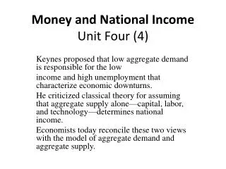
Money and National Income Unit Four (4). Keynes proposed that low aggregate demand is responsible for the low income and high unemployment that characterize economic downturns.

Money and National Income Unit Four (4)
E N D
Presentation Transcript
Money and National IncomeUnit Four (4) Keynes proposed that low aggregate demand is responsible for the low income and high unemployment that characterize economic downturns. He criticized classical theory for assuming that aggregate supply alone—capital, labor, and technology—determines national income. Economists today reconcile these two views with the model of aggregate demand and aggregate supply.
Money and National IncomeUnit Four (4) IS-LM model The goal of the model is to show what determines national income for a given price level. There are two ways to interpret this exercise. We can view the IS–LM model as showing what causes income to change in the short run when the price level is fixed because all prices are sticky. Or we can view the model as showing what causes the aggregate demand curve to shift.
Money and National IncomeUnit Four (4) IS stands for “investment’’ and “saving,’’ and the IS curve represents what’s going on in the market for goods and services. LMstands for “liquidity’’ and “money,’’ and the LM curve represents what’s happening to the supply and demand for money. Because the interest rate influences both investment and money demand, it is the variable that links the two halves of the IS–LM model. The model shows how interactions between the goods and money markets determine the position and slope of the aggregate demand curve and, therefore, the level of national income in the short run.
The Goods Market and the IS Curve Keynesian cross In The General Theory Keynes proposed that an economy’s total income was, in the short run, determined largely by the spending plans of households, businesses, and government. The more people want to spend, the more goods and services firms can sell. The more firms can sell, the more output they will choose to produce and the more workers they will choose to hire. Keynes believed that the problem during recessions and depressions was inadequate spending. The Keynesian cross is an attempt to model this insight.
The Goods Market and the IS Curve We begin our derivation of the Keynesian cross by drawing a distinction between actual and planned expenditure. Actual expenditure is the amount households, firms, and the government spend on goods and services, which is equals the economy’s gross domestic product (GDP). Planned expenditure is the amount households, firms, and the government would like to spend on goods and services.
The Goods Market and the IS Curve The Keynesian Cross PE and Y Actual exp = Planned Exp Y=PE Planned Exp PE=C+I+G 0 Equil income Income, Output
The Goods Market and the IS Curve The Interest Rate, Investment, and the IS Curve. Planned investment depends on the rate of interest, r. I = I(r) Interest rate is the cost of borrowing to finance investment projects, an increase in the interest rate reduces planned investment. As a result, the investment function slopes downward.
The Goods Market and the IS Curve Deriving the IS Curve Panel (a) shows the investment function: an increase in the interest rate from r1 to r2 reduces planned investment from I(r1) to I(r2). Panel (b) shows the Keynesian cross: a decrease in planned investment from I(r1) to I(r2) shifts the planned-expenditure function downward and thereby reduces income from Y1 to Y2. Panel (c) shows the IS curve summarizing this relationship between the interest rate and income: the higher the interest rate, the lower the level of income.
The Goods Market and the IS Curve How Fiscal Policy Shifts the IS Curve The IS curve shows us, for any given interest rate, the level of income that brings the goods market into equilibrium. As we learned from the Keynesian cross, the equilibrium level of income also depends on government spending G and taxes T. The IS curve is drawn for a given fiscal policy; that is, when we construct the IS curve, we hold G and T fixed. When fiscal policy changes, the IS curve shifts.
The Goods Market and the IS Curve How Fiscal Policy Shifts the IS Curve An Increase in Government Purchases Shifts the IS Curve Outward Panel (a) shows that an increase in government purchases raises planned expenditure. For any given interest rate, the upward shift in planned expenditure of ΔG leads to an increase in income Y of ΔG/(1 − MPC). Therefore, in panel (b), the IS curve shifts to the right by this amount.
The Goods Market and the IS Curve In summary, the IS curve shows the combinations of the interest rate and the level of income that are consistent with equilibrium in the market for goods and services. The IS curve is drawn for a given fiscal policy. Changes in fiscal policy that raise the demand for goods and services shift the IS curve to the right. Changes in fiscal policy that reduce the demand for goods and services shift the IS curve to the left.
The Money Market and the LM Curve The LM curve plots the relationship between the interest rate and the level of income that arises in the market for money balances. The Theory of Liquidity Preference The theory of liquidity preference assumes there is a fixed supply of real money balances, That is
The Money Market and the LM Curve The money supply M is an exogenous policy variable chosen by a central bank. The price level P is also an exogenous variable in this model. (We take the price level as given because the IS– LM model—our ultimate goal in this chapter—explains the short run when the price level is fixed.) These assumptions imply that the supply of real money balances is fixed and, in particular, does not depend on the interest rate
The Money Market and the LM Curve The theory of liquidity preference state that the interest rate is one determinant of how much money people choose to hold. The underlying reason is that the interest rate is the opportunity cost of holding money: it is what you forgo by holding some of your assets as money, which does not bear interest, instead of as interest-bearing bank deposits or bonds. When the interest rate rises, people want to hold less of their wealth in the form of money. We can write the demand for real money balances as (M/P)d = L(r),
The Money Market and the LM Curve The Theory of Liquidity Preference The supply and demand for real money balances determine the interest rate. The supply curve for real money balances is vertical because the supply does not depend on the interest rate. The demand curve is downward sloping because a higher interest rate raises the cost of holding money and thus lowers the quantity demanded. At the equilibrium interest rate, the quantity of real money balances demanded equals the quantity of real money balance supplied.
The Money Market and the LM Curve The Theory of Liquidity Preference Interest rate r L(r) m/p real money balances
The Money Market and the LM Curve The Theory of Liquidity Preference How does the interest rate get to this equilibrium of money supply and money demand? The adjustment occurs because whenever the money market is not in equilibrium, people try to adjust their portfolios of assets and, in the process, alter the interest rate. For instance, if the interest rate is above the equilibriumlevel, the quantity of real money balances supplied exceeds the quantity demanded. Individuals holding the excess supply of money try to convert some of their non- interest-bearing money into interest-bearing bank deposits or bonds.
The Money Market and the LM Curve The Theory of Liquidity Preference Banks and bond issuers, who prefer to pay lower interest rates, respond to this excess supply of money by lowering the interest rates they offer. Conversely, if the interest rate is below the equilibrium level, so that the quantity of money demanded exceeds the quantity supplied, individuals try to obtain money by selling bonds or making bank withdrawals. To attract now-scarcer funds, banks and bond issuers respond by increasing the interest rates they offer. the interest rate reaches the equilibrium level, at which people are content with their portfolios of monetary and nonmonetary assets
Income, Money Demand, and the LM Curve How does a change in the economy’s level of income Y affect the market for real money balances? The level of income affects the demand for money. When income is high, expenditure is high, so people engage in more transactions that require the use of money. Thus, greater income implies greater money demand. We can express these ideas by writing the money demand function as (M/P)d = L(r, Y ). The quantity of real money balances demanded is negatively related to the interest rate and positively related to income.
Income, Money Demand, and the LM Curve What happens to the equilibrium interest rate when the level of income Changes? For example, consider what happens in when income increases from Y1 to Y2. As panel (a) illustrates, this increase in income shifts the money demand curve to the right. With the supply of real money balances unchanged, the interest rate must rise from r1 to r2 to equilibrate the money market. Therefore, according to the theory of liquidity preference, higher income leads to a higher interest rate. The LM curve summarizes this relationship between the level of income and the interest rate. Each point on the LM curve represents equilibrium in the money market, and the curve illustrates how the equilibrium interest rate depends on the level of income. The higher the level of income, the higher the demand for real money balances, and the higher the equilibrium interest rate. For this reason, the LM curve slopes upward.
Income, Money Demand, and the LM Curve How Monetary Policy Shifts the LM Curve Let us use the theory of liquidity preference to understand how monetary policy shifts the LM curve. Suppose that the Bank of Namibia decreases the money supply from M1 to M2, which causes the supply of real money balances to fall from M1/P to M2/P. Holding constant the amount of income and thus the demand curve for real money balances, we see that a reduction in the supply of real money balances raises the interest rate that equilibrates the money market. Hence, a decrease in the money supply shifts the LM curve upward.
Income, Money Demand, and the LM Curve In summary, the LM curve shows the combinations of the interest rate and the level of income that are consistent with equilibrium in the market for real money balances. The LM curve is drawn for a given supply of real money balances. Decreases in the supply of real money balances shift the LM curve upward. Increases in the supply of real money balances shift the LM curve downward
The short-run equilibrium We now have all the pieces of the IS–LM model. The two equations of this model are Y = C(Y − T ) + I(r) +G IS, M/P = L(r, Y ) LM. The model takes fiscal policy G and T, monetary policy M, and the price Level P as exogenous. Given these exogenous variables, the IS curve provides the combinations of r and Y that satisfy the equation representing the goods market, and the LM curve provides the combinations of r and Y that satisfy the equation representing the money market.
The short-run equilibrium We now have all the pieces of the IS–LM model. Interest rate LM IS Income
The short-run equilibrium A numerical example to practice Consider the following short-run model of closed economy Good Market C=10+0.1Yd I = 5-5r G = 20; T = 10 Money Market M = 10 P = 2 L(Y,r) = Y –r We will start by constructing IS and LM equations Y = C(Y − T ) + I(r) +G IS equation
The short-run equilibrium A numerical example to practice Y = C(Y − T ) + I(r) +G IS equation Y = 10+0.1Y-0.1T+5-5r+20 Y-0.1Y=34-5r Y(1-0.1)=34-5r 0.9Y/0.9=34/0.9-5r/0.9 Y=37.8-5.6r this is IS equation
The short-run equilibrium A numerical example to practice M/P = L(r, Y ) LM equation 10/2=Y-r 5=Y-r Y=5+r this is LM equation
The short-run equilibrium A numerical example to practice Plotting IS-LM curves 6.3 LM 5 IS 5 10 38
The short-run equilibrium A numerical example to practice Equilibrium interest and income We equate IS and LM equations 37.8-5.6r=5+r and we find the value of r r=5 We substitute the value of r into IS or LM equation to get the Value of Y. Y=37.8-5.6(5) or Y=5+5 Y=10 or Y =10