Download
1 / 50
500 likes | 657 Views
Shape similarity and Visual Parts. Longin Jan Latecki Temple Univ., latecki@temple.edu In cooperation with Rolf Lakamper (Temple Univ.), Dietrich Wolter (Univ. of Bremen). Object Recognition Process:. Source: 2D image of a 3D object. Object Segmentation. Contour Extraction. Evolution.

E N D
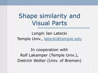
Shape similarity and Visual Parts Longin Jan Latecki Temple Univ., latecki@temple.edu In cooperation with Rolf Lakamper (Temple Univ.), Dietrich Wolter (Univ. of Bremen)
Object Recognition Process: Source: 2D image of a 3D object Object Segmentation Contour Extraction Evolution Contour Segmentation Matching: Correspondence of Visual Parts
What is this talk about ? Comparison of object shape based on object contours • Object contours are naturally obtained in Computer Vision, Robot Navigation, and other applications as polylines (polygonal curves). • • Shape similarity reduces to similarity of polylines. • Shape similarity of polylines is not so simple: • simple 1-1 vertex correspondence does not work • a scale problem
Cognitive Similarity Requirements • Since polylines are obtained as boundary parts of objects in usually noisy sensor data (e.g., digital images): • two similar polylines do not need to have the same number of vertices, i.e., do not have to be of comparable level of detail, • do not have to be of comparable size, • may have only a subpart that is similar and that has a significant contribution to their shape = visual part
Comparable level of detail (1) • It can be achieved in the context of • a single object or • a group of objects (e.g., a query and a goal shape) • How can we achieve a comparable level of detail for • all objects if we treat each object separately? • By placing each object on the same level of the • Scale Space hierarchy.
Discrete Curve Evolution (DCE) • We achieve a comparable level of detail with DCE. • Before a similarity measure is applied, the shape of objectsis simplified by DCE in order to • reduce influence of noise, • simplify the shape by removing irrelevant shape featureswithout changing relevant shape features.
Discrete Curve Evolution (DCE) It yields a sequence: P=P0, ..., Pm Pi+1 is obtained from Pi by deleting the vertices of Pi that have minimal relevance measure K(v, Pi) = |d(u,v)+d(v,w)-d(u,w)| v v > w w u u
Discrete Curve Evolution: Preservation of position, no blurring
Discrete Curve Evolution: mathematical properties Convexity Theorem (trivial) Discrete curve evolution (when applied to a polygon) converges toa convex polygon. Continuity Theorem (nontrivial) Discrete curve evolution is continuous. L. J. Latecki, R.-R. Ghadially, R. Lakämper, and U. Eckhardt: Continuity of the discrete curve evolution. Journal of Electronic Imaging 9, pp. 317-326, 2000. Polygon Recovery (nontrivial) DCE allows to recover polygons from their digital images. L.J. Latecki and A. Rosenfeld: Recovering a Polygon form Noisy Data. Computer Vision and Image Understanding (CVIU) 86, 1-20, 2002.
Comparable level of detail for DCE (=stop condition) is based on a threshold on the relevance measure
Comparable level of detail for DCE is based on a threshold on the relevance measure
Scale Space Approaches to Curve Evolution • reaction-diffusion PDEs • polygonal analogs of the PDE-evolution(Bruckstein et al. 1995) • approximation (e.g., Bengtsson and Eklundh 1991) • Main differences: • [to 1, 2:] Each vertex of the polygon is movedat a single evolution step,whereas in our approachthe remaining vertices do not change their positions. • [to 1, 3:] Our approach is parameter-free(we only need a stop condition)
(3) Local similarity • We need local similarity measure, • i.e., we need to compare polylines but not polygons. • Global similarity measures fail at: • - partial visibility (occlusion) • - not uniformly distributed noise • - actually everything that occurs under • real conditions
Local similarity A simple solution to local similarity measure: Given a target polylineT, find the most similar part P of polyline Q. Consider all subpolylines of Q combinatorial explosion We consider only all connected subsets P of Q, O(n²) in the number of vertices n of Q. However, a connected subset P may be a distorted version of T.
Optimal Shape Similarity • The optimal similarity of P to T is the similarity of modified P to T, where modified P is P with all features that make P distinct from T removed. s is a global similarity measure Consider all subpolylines of P combinatorial explosion
All shape similarity measures presented in the literature are global measures. • Although they can be applied to local parts, they are not optimal.
Presented approach A two-step solution: • We consider only all connected subsets P of Q, O(n²),n vertices of Q. • We use a greedy algorithm to compute optimal similarity, O(n²),n vertices of P. We need a global similarity measure s.
Shape Similarity in Tangent Space A polyline P is mapped to its turn angle function T(P)in the tangent space the height of each step shows the turn-angle, monotonically increasing intervals represent convex arcs, height-shifting corresponds to rotation, the resulting curve can be interpreted as 1D signal
Shape Comparison: Measure Drawback: not adaptive to unequally distributed noise
Shape Comparison: Contour Segmentation Solution: use this measure only locally, i.e., apply only to corresponding parts:
Correspondence of visual parts: non-rigid deformation L. J. Latecki and R. Lakämper: Shape Similarity Measure Based on Correspondence of Visual Parts. IEEE Trans. Pattern Analysis and Machine Intelligence 22, 2000. L. J. Latecki and R. Lakämper: Application of Planar Shape Comparison to Object Retrieval in Image Databases. Pattern Recognition 35, 2002.
Partial Shape Matching • This shape similarity measure works fine if the whole contour • is given: • Great performance in the MPEG-7 competition • Life web-based shape search engine • Can it be applied when only contour parts are given? • Yes, but only in the context of optimal shape similarity.
Subpart Selection • We can use sliding window on the contour of the object Q • to find a given target part T. • However, we cannot expect to cut part P of Q that exactly • corresponds to T, due to • imperfect size of the window • noise and change of view point • scale selection. Q T Therefore, a similarity measure must be able to overlook parts of Q whose shape is irrelevant w.r.t. Q.
Matching and Simplification The main idea of the proposed computation of the optimal similarity is shape matching and simplification similar to DCE in one process. The main idea: We recursively remove a vertices of P to obtain P’ such that P’is the most similar to T. os(T,P)= global minimum of s(T,P’). We achieve a comparable level of detail (1)for polyline P in the context of target T. Observe that this approach also solves the stop condition problem (DCE is applied to each object separately).
Matching and Simplification II Given a target T and a polyline P. os(T,P) = global minimum S(T,P’) + S(P’,P), where and are weights. The simplest weight assignment is = 1 and =0.
Applications • Shape-based object recognition • Retrieval in image and video databases • Object tracking • Shape-based tracking of objects in laser scans • Robot mapping • Robot localization in top view maps
Shape-based tracking of objects in laser scans An example top view image of LRF scan data
Shape-based tracking of objects in laser scans Row scan data (left) is segmented into polyline (right)
Matching scans by shape Since shape may be very simple, we also use cyclic order and proximity information
Shape-based tracking of objects in laser scansBuilding a global map Demo movie Why go beyond the simple proximity of points computed by minimizing the least squared distance of all points? Robot may slip or turn (unconsciously): Shape and order of polylines remain similar even if the displacement is significant
Robot mapping and localization • Shape similarity useful for: • globally consistent mapping • localization when odometry is not given or unreliable
Future Work Learning of visual parts: How to select the most distinctive parts of objects? Our approach is based on statistics and our shape similaritymeasures: We use statistical methods to find the smallest possible setof most different parts within a given class of objectsand the smallest possible set of most separating parts among different object classes. Previous approaches to find visual parts are based on differential geometry. They are static in that the parts will be always the same for different classes of objects. Our approach is dynamic: selected parts depend on the objects seen.