Download
1 / 38
380 likes | 412 Views
Explore innovative approaches in data assimilation, balancing linearization with Bayesian principles for optimal results. Learn about geometric tangent linear approximations and mixed lognormal-Gaussian techniques.

E N D
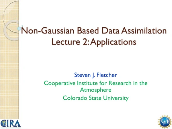
Non-Gaussian Based Data AssimilationLecture 2: Applications Steven J. Fletcher Cooperative Institute for Research in the Atmosphere Colorado State University
Overview of Lecture Do we linearize the Bayesian problem or do we find the Bayesian Problem for the linear increment? Geometric Tangent Linear Approximation Mixed Multiplicative-Additive Incremental 4DVAR Lognormal Detection Algorithm Mixed Lognormal-Gaussian Mixing Ratio – Temperature retrievals Optimal Regions for Descriptive Statistics for Lognormal Based DA Chaotic Signal with Newton-Raphson solver and Lognormal DA JCSDA 2015 Colloquium on Satellite DA
Do we linearize the Bayesian problem or do we find the Bayesian Problem for the linear increment? The first version of a incremental approach for a lognormal based variational data assimilation method appears in Song et al., (2012). Their starting point was to define an increment as Where the circle represents the Hadamard multiplication operator which is a component wise vector multiplication. This increment is then substituted into the background component of the lognormal cost function which results in Which has linearized the cost function by removing the logarithms but this is not consistent with keeping the probability distributions equal on either side of the equals side as dictated by the uniqueness theorem for moment generating functions. If we assume that the true state is a lognormally distributed random variable (RV) and that the background is also a lognormally distributed RV then we require the exponential term to also be a lognormal RV. This can only occur if is a Gaussian RV. Therefore, for us to be able to optimize the increments we need to be solving a Gaussian cost function for it. In Song et al., (2012) they present results from both the linearized version which did not work well, which is to be expected as the Bayesian problem is not consistent, but when they used what they refer to as the median approach, which is the equation above with out the inner product, they were able to show better results than assuming a Gaussian based approach. The motivation in Song et al., (2012) for a lognormal approach was to avoid negative values for positive definite variables, that the Gaussian approach kept giving. Song, H. C., A. Edwards, A. M. Moore and J. Fiechter, 2012: Incremental four-dimensional variational data assimilation of positive-definite oceanic variables using a logarithmic transformation. Ocean Modell., 54-55, 1—17. JCSDA 2015 Colloquium on Satellite DA
Do we linearize the Bayesian problem or do we find the Bayesian Problem for the linear increment? In Fletcher and Jones (2014) and alternative incremental formulation was proposed. The alternative formulation focused upon keeping the problem lognormal as much as possible. Therefore, this implied that the formulation linking the true state to the background state needed to be lognormal and not be such that it linearized the cost function. The definition that keeps the problem lognormally consistent is This now implies that for both sides of the equal sign to be lognormal, if the true state is assumed to be a lognormal RV and so is the background, must also be a lognormal RV. Substituting this expression into the full field background component of the cost function results in Which is a lognormal cost function for the mode of a lognormal distribution. Fletcher, S.J. and A. S. Jones, 2014: Multiplicative and additive incremental variational data assimilation for mixed lognormal-Gaussian errors. Mon. Wea. Rev., 142, 2521—2544. JCSDA 2015 Colloquium on Satellite DA
Geometric Tangent Linear Approximation The question now is how to linearize the observational component with respect to a multiplicative increment? That is to say we need to linearize In Fletcher and Jones (2014) it is shown that we can use the same theory behind a tangent linear approximation with an additive increment but now using an multiplicative increment. If we consider the diagrams below The plot on the left is to illustrate how we obtain the additive tangent linear approximation, whilst the figure on the right is to illustrate how we can obtain an expression involving multiplicative increments. JCSDA 2015 Colloquium on Satellite DA
Geometric Tangent Linear Approximation This then allows us to be able to use standard derivative results for a multiplicative increment. Which means that for lognormal 3DVAR the observation operator can be approximated by And for 4DVAR by JCSDA 2015 Colloquium on Satellite DA
Mixed Multiplicative-Additive Incremental 4DVAR As we do not live in a just Gaussian or lognormal world, we have to combine the two approaches, as we have done for the full field (Fletcher, 2010). We therefore define our incremental vector as This then gives the following 4DVAR cost function (Fletcher and Jones, 2014). JCSDA 2015 Colloquium on Satellite DA
Mixed Multiplicative-Additive Incremental 4DVAR JCSDA 2015 Colloquium on Satellite DA
Mixed Multiplicative-Additive Incremental 4DVAR The Lorenz model is given by the following non-linear system of three ordinary differential equation The system is linearized and then discretized using the modified Euler scheme. The adjoint of this scheme is calculated analytically. The minimization of the cost function is achieved through the fminsearch routine in MATLAB which uses a Nelder-Mead algorithm. The observations are calculated by adding random perturbations from a Gaussian distribution, (x and y components) and multiplying perturbations from a lognormal distribution (z component) to the true model run. JCSDA 2015 Colloquium on Satellite DA
Mixed Multiplicative-Additive Incremental 4DVAR Results for 20 cycles of 100ts with few accurate obs JCSDA 2015 Colloquium on Satellite DA
Mixed Multiplicative-Additive Incremental 4DVAR JCSDA 2015 Colloquium on Satellite DA Results with same window lengths and same number of obs but less accurate
Mixed Multiplicative-Additive Incremental 4DVAR Results for same number of assimilation windows but with accurate observations every other time step JCSDA 2015 Colloquium on Satellite DA
Mixed Multiplicative-Additive Incremental 4DVAR Results for same number of assimilation windows but with accurate observations every other time step JCSDA 2015 Colloquium on Satellite DA
Comparison to a full Gaussian incremental system These results are from Fletcher and Jones (2014) paper where here we are presenting results from two of the experiments, the first to highlight where the two systems are similar and the case where the lognormal converges but the Gaussian does not. Gaussian approximates the lognormal. Small observational error variance Lognormal stays stable whilst Gaussian does not JCSDA 2015 Colloquium on Satellite DA
Lognormal Detection Algorithm There is a lot of growing evidence that the distribution of certain atmospheric, and oceanic fields, do not have a Gaussian distribution continuously throughout the year. Therefore the question becomes, how can we know when to use a lognormal or a Gaussian based data assimilation system? Dr. Anton Kliewer, a NSF funded postdoctoral fellow at CIRA/CSU has been developing an algorithm that is based upon a composite of three statistical tests which determine if the data that you are testing are presenting a lognormal signal, a Gaussian signal or a non-Gaussian signal that is not a lognormal but does not determine this other distribution. Similar work to detect non-Gaussian signals is being undertaken at Météo-France. JCSDA 2015 Colloquium on Satellite DA
Lognormal Detection Algorithm Kliewer, A. J, S. J. Fletcher, J. M. Forsythe and A. S. Jones 2015a: Identifying Non-normal and lognormal characteristics of temperature, mixing ratio, surface pressure, and winds for data assimilation systems. Submitted to Nonlinear Processes in the Geosciences Hypothesis Tests: Shapiro-Wilk – combines the information that is contained in the normal probability plot with the information obtained from the estimator of the standard deviation of the sample. Jarque-Bera– a goodness-of-fit test of whether sample data have the skewness and kurtosis matching a normal distribution. Chi-Squared Goodness-of-Fit – determines whether there is a significant difference between the expected frequencies and the observed frequencies from a probability distribution. Composite – combination of the previous three tests. (Kliewer et al, 2015a) JCSDA 2015 Colloquium on Satellite DA
Lognormal Detection Algorithm For Shapiro-Wilk and Jarque-Bera, the null hypothesis is that the data comes from a Gaussian distribution. The alternative hypothesis is the data does not come from a Gaussian distribution. For the Chi-squaredthe null hypothesis is that the data comes from a lognormal distribution.The alternative hypothesis is the data does not come from a lognormal distribution. The composite test combines these results – a positive result (red on images) indicates that the data does not come from a Gaussian distribution (as determined by Shapiro-Wilk and Jarque-Bera) and it does come from a lognormal distribution (as determined by Chi-squared). A negative result (blue on image) indicates that either Shapiro-Wilk or Jarque-Beradetermined the data to come from a Gaussian distribution, or the Chi-squared determined the data does not come from a lognormal distribution. All tests conducted at the α=0.01 significance level (99% confidence). JCSDA 2015 Colloquium on Satellite DA
For this study one year (2005) of Global Forecast System 0 hr forecasts from the 0z runs of mixing ratio were treated as observations of the ``true state'' and analyzed using statistical hypothesis testing procedures. Global 500hPa mixing ratio JCSDA 2015 Colloquium on Satellite DA
Continental United States JCSDA 2015 Colloquium on Satellite DA
Gulf of Mexico JCSDA 2015 Colloquium on Satellite DA
Off the coast of Africa JCSDA 2015 Colloquium on Satellite DA
North Atlantic/Mid-Latitudes JCSDA 2015 Colloquium on Satellite DA
Same analysis but now with the 6 hour forecast which is used as the first guess for the next assimilation cycle. JCSDA 2015 Colloquium on Satellite DA
Surface Pressure Non-Gaussian Detection Indicators of when surface pressure by three month groupings had a non-Gaussian signal, but not a lognormal signal. JCSDA 2015 Colloquium on Satellite DA
Surface Pressure Non-Gaussian Detection A composite for the whole of 2005 and broken down by 3 month groupings to detect non-Gaussian signals for surface pressure. JCSDA 2015 Colloquium on Satellite DA
Mixed Lognormal-Gaussian Mixing Ratio – Temperature Retrievals Engelen, R. J. and G.L. Stephens, 1999: Characterization of water-vapour retrievals from TOVS/HIRS, and SSM/T-2 measurement. Q. J. Roy. Meteorol. Soc., 125, 331—351. Liebe, H.J., 1989: MPM – An atmospheric millimeter-wave propagation model. Int. J. Infrared and Millimeter Waves, 10, 631—650. At CIRA we have implemented the full-field mixed lognormal-Gaussian theory into the CIRA1-Dimensional Optimal Estimator (C1DOE). C1DOE is a microwave retrieval system that retrieves emissivities, mixing-ratio and temperature. For the experiments that we performed we updated the background error covariance matrices for both the Gaussian and mixed formulations. These updates were calculated from GDAS data for the month of September 2005. We have adapted the retrieval system to also perform the transform approach as well as the mixed formulation. C1DOE is a microwave radiance/brightness temperature based retrieval system using the radiative transfer theory set out in Liebe (1989) and the subsequent revisions in 1992. A good description of C1DOE formulations can be found in Engelen and Stephens (1999). The retrievals are performed on 7 vertical levels at 1000hPa, 850hPa, 700hPa, 500hPa, 200hPa and 100hPa. The experiment were ran for 10 days from 09/01/2005 – 09/10/2005. The cost function is solved using a Newton-Raphson Solver where we are using the correct Jacobians and are inverting the analytical Hessian matrices. JCSDA 2015 Colloquium on Satellite DA
Mixed Lognormal-Gaussian Mixing Ratio – Temperature Retrievals Field of View for the experiments presented in Kliewer et al., (2015b) where a non-Gaussian signal for moisture had been detected near the coast of Japan for this year from GPS station data. Kliewer, A.J., S.J. Fletcher, A.S. Jones and J.M. Forsythe, 2015b: Comparison of Gaussian, Logarithmic transform and Mixed Gaussian-Lognormal distribution-based 1DVAR Microwave Temperature-Water Vapor Mixing Ratio. Under Revision for Q. J. Roy. Meteorol. Soc. JCSDA 2015 Colloquium on Satellite DA
Mixed Lognormal-Gaussian Mixing Ratio – Temperature Retrievals Comparisons of the three retrieval methods against the Microwave Surface and Precipitation Products Systems (MSPPS) TPW product. Solid is the mixed approach, dot-dashed is the transform and the dashed is the Gaussian. JCSDA 2015 Colloquium on Satellite DA
Mixed Lognormal-Gaussian Mixing Ratio – Temperature Retrievals AMSU-B Channel 4 (183 ± 3GHz) (Water Vapor Channel in the troposphere) Final Innovations JCSDA 2015 Colloquium on Satellite DA
Mixed Lognormal-Gaussian Mixing Ratio – Temperature Retrievals AMSU-A Channel 6 (54.4GHz) (Temperature Channel in the troposphere) Final Innovations JCSDA 2015 Colloquium on Satellite DA
Optimal Regions for Descriptive Statistics for Lognormal Based DA Fletcher, S. J., A. J. Kliewer and A. S. Jones, 2015: Quantification of optimal choices of parameters in lognormal variational data assimilation and their chaotic behavior. Submitted to SIAM J. Uncertainty Quantification. During the implementation of a set of synthetic experiments with C1DOE to ascertain the accuracy of the three different approaches for a know true solution, it became apparent that something was affecting the performance of the modal based approach in that it could not beat the median approach even though we thought the problem had been set up so that the mode should have been the optimal estimator. We ran a series of experiments with a univariate formulation with the lognormal cost function and used a Newton-Raphson solver to simulate the processes in C1DOE. During these experiments we discovered 4 important findings relative to the performance of a lognormal modal based variational problem (Fletcher et al., 2015). The three descriptive statistics, mean, median and mode, had regions relative to the apriori state such that they were the statistic that minimized the errors. There existed a value for the apriori state for each statistic such that the minimum of the cost function was at the true state. That if a apriori state was close to this optimal value then the Newton-Raphson solver became chaotic and incredibly sensitive to the first guess to the solver. The apriori state should not be the best approximation to the true state for the lognormal modal approach but rather to This is because If the apriori state is close to the true state the median is optimal in minimizing the errors whilst if the apriori state is close then the mode is the optimal statistic. JCSDA 2015 Colloquium on Satellite DA
Optimal Regions for Descriptive Statistics for Lognormal Based DA Optimal values are Mean: Median: Mode: Plot of absolute error for different values for the apriori state for different lognormal descriptive statistic cost functions. JCSDA 2015 Colloquium on Satellite DA
Optimal Regions for Descriptive Statistics for Lognormal Based DA Impact of the variance on the range where the median minimizes the error. JCSDA 2015 Colloquium on Satellite DA
Chaotic Signal with Newton-Raphson solver and Lognormal DA It was when we introduced a measurement error to determine what the optimal value for the apriori state (or the observational and background variances) that we started to detect that there was something happening to the accuracy of the solution of the modal approach with the Newton-Raphson solver with respect to the choice of first guess to the solver!! JCSDA 2015 Colloquium on Satellite DA
Chaotic Signal with Newton-Raphson solver and Lognormal DA Upon a series of trial and error experiments with the first guess values we started to see that the point where we needed to start from to ensure accuracy of in our solution or better was changing, but that this value at every decimal point was changing!!! We would get to a value at each decimal point that if we went past that number at that decimal point we would lose 3 to 4 figures of accuracy!! To investigate this feature we ran do loops over first guess to the Newton-Raphson solver stepping by 0.001 and for measurement errors stepping at 0.001 from 0 to 1. This is what we found JCSDA 2015 Colloquium on Satellite DA
Chaotic Signal with Newton-Raphson solver and Lognormal DA JCSDA 2015 Colloquium on Satellite DA
Chaotic Signal with Newton-Raphson solver and Lognormal DA To investigate how wide spread this chaotic affect was we changed the values for the optimal apriori state to be 99%, 99.9%, 99.999% and 99.9999% of optimal and what we found was worrying. JCSDA 2015 Colloquium on Satellite DA
Chaotic Signal with Newton-Raphson solver and Lognormal DA This signal is not only present when the apriori state is optimized for measurement error. It is also present when the apriori state is optimized for representative errors as well as in the Gaussian formulation and the incremental lognormal formulation. A different fractal appears for each and for different true states as well as different background and observational errors. It is also present when the background or the observational errors are optimized to correct for the other incorrect statistics to ensure that the minimum of the cost function is at the true state. This patterns are referred to as Newton-Fractals and occur when the quadratic convergence breaks down. JCSDA 2015 Colloquium on Satellite DA