Dynamic Simulation : Lagrange’s Equation
Dynamic Simulation : Lagrange’s Equation. Objective The objective of this module is to derive Lagrange’s equation, which along with constraint equations provide a systematic method for solving multi-body dynamics problems. Section 4 – Dynamic Simulation Module 6 – Lagrange’s Equation

Dynamic Simulation : Lagrange’s Equation
E N D
Presentation Transcript
Dynamic Simulation: • Lagrange’s Equation Objective • The objective of this module is to derive Lagrange’s equation, which along with constraint equations provide a systematic method for solving multi-body dynamics problems.
Section 4 – Dynamic Simulation Module 6 – Lagrange’s Equation Page 2 • Problems in dynamics can be formulated in such a way that it is necessary to find the stationary value of a definite integral. • Lagrange (1736-1813) created the Calculus of Variations as a method for finding the stationary value of a definite integral. He was a self taught mathematician who did this when he was nineteen. • Euler (1707-1783) used a less rigorous but completely independent method to do the same thing at about the same time. • They were both trying to solve a problem with constraints in the field of dynamics. Calculus of Variations
Section 4 – Dynamic Simulation Module 6 – Lagrange’s Equation Page 3 Leonhard Euler Joseph-Louis Lagrange Euler and Lagrange 1707-1783 1736-1813 http://en.wikipedia.org/wiki/Leonhard_Euler http://en.wikipedia.org/wiki/Lagrange
Section 4 – Dynamic Simulation Module 6 – Lagrange’s Equation Page 4 Hamilton’s Principle states that the path followed by a mechanical system during some time interval is the path that makes the integral of the difference between the kinetic and the potential energy stationary. Hamilton’s Principle L=T-V is the Lagrangian of the system. Tand V are respectively the kinetic and potential energy of the system. The integral, A, is called the action of the system.
Section 4 – Dynamic Simulation Module 6 – Lagrange’s Equation Page 5 Hamilton’s Principle is also called the “Principle of Least Action” since the paths taken by components in a mechanical system are those that make the Action stationary. Principle of Least Action Action
Section 4 – Dynamic Simulation Module 6 – Lagrange’s Equation Page 6 • The application of Hamilton’s Principle requires that we be able to find the stationary value of a definite integral. • We will see that finding the stationary value of an integral requires finding the solution to a differential equation known as the Lagrange equation. • We will begin our derivation by looking at the stationary value of a function, and then extend these concepts to finding the stationary value of an integral. Stationary Value of an Integral
Section 4 – Dynamic Simulation Module 6 – Lagrange’s Equation Page 7 • A function is said to have a “stationary value” at a certain point if the rate of change of the function in every possible direction from that point vanishes. • In this example, the function has a stationary point at x=x1. At this point, its first derivative is equal to zero. y Stationary Value of a Function y=f(x) y1 x1 x
Section 4 – Dynamic Simulation Module 6 – Lagrange’s Equation Page 8 In 3D the rate of change of the function in any direction is zero at a stationary point. Note that the stationary point is not necessarily a maximum or a minimum. 3D Stationary Points
Section 4 – Dynamic Simulation Module 6 – Lagrange’s Equation Page 9 y • f(x) is an arbitrary function that satisfies the boundary conditions at a and b. • g(x) can be made infinitely close to f(x) by making the parameter e infinitesimally small. Variation of a Function dy Candidate Path y=f(x) dy dx Actual Path x a x+dx x b
Section 4 – Dynamic Simulation Module 6 – Lagrange’s Equation Page 10 • The Calculus of Variations considers a virtual infinitesimal change of function y = f(x). • The variation dy refers to an arbitrary infinitesimal change of the value of yat the point x. • The independent variable x does not participate in the process of variation. y Meaning of dy dy y=f(x) dy dx x a x+dx x b
Section 4 – Dynamic Simulation Module 6 – Lagrange’s Equation Page 11 In the calculus of variations, the derivative of the variation and the variation of the derivative are equal. Variation of a Derivative Variation of the Derivative Derivative of the Variation The order of operation is interchangeable.
Section 4 – Dynamic Simulation Module 6 – Lagrange’s Equation Page 12 In the calculus of variations, the variation of a definite integral is equal to the integral of the variation. Integral of a Variation Variation of an Integral Variation of a Definite Integral The order of operation is interchangeable.
Section 4 – Dynamic Simulation Module 6 – Lagrange’s Equation Page 13 The specific definite integral that we want to find the stationary value of is the Action from Hamilton’s Principle. It can be written in functional form as Specific Definite Integral qiare the generalized coordinates used to define the position and orientation of each component in the system. The actual path that the system will follow will be the one that makes the definite integral stationary.
Section 4 – Dynamic Simulation Module 6 – Lagrange’s Equation Page 14 The stationary value of an integral is found by setting its variation equal to zero. Euler-Lagrange Equation Derivation A first order Taylor’s Series was used in the last step. For an arbitrary value of e,
Section 4 – Dynamic Simulation Module 6 – Lagrange’s Equation Page 15 The second integral is integrated by parts. Integration by Parts Substitutions Euler-Lagrange Equation Derivation f is equal to zero at t1 and t2.
Section 4 – Dynamic Simulation Module 6 – Lagrange’s Equation Page 16 The only way that this definite integral can be zero for arbitrary values of fiis for the partial differential equation in parentheses to be zero at all values of x in the interval t1to t2. Euler-Lagrange Equation Derivation or Lagrange’s equation
Section 4 – Dynamic Simulation Module 6 – Lagrange’s Equation Page 17 Finding the stationary value of the Action, A, for a mechanical system involves solving the set of differential equations known as Lagrange’s equation. Euler-Lagrange Summary Solving these equations Makes this integral stationary
Section 4 – Dynamic Simulation Module 6 – Lagrange’s Equation Page 18 • Although the derivation of Lagrange’s equation that provides a solution to Hamilton’s Principle of Least Action, seems abstract, its application is straight forward. • Using Lagrange’s equation to derive the equations of motion for a couple of problems that you are familiar with will help to introduce their application. Examples
Section 4 – Dynamic Simulation Module 6 – Lagrange’s Equation Page 19 Governing Equations Mathematical Operations y Vibrating Spring Mass Example m k y is measured from the static position. Equation of Motion
Section 4 – Dynamic Simulation Module 6 – Lagrange’s Equation Page 20 Governing Equations Mathematical Operations m Falling Mass Example g y x Equation of Motion
Module Summary Section 4 – Dynamic Simulation Module 6 – Lagrange’s Equation Page 21 • Lagrange’s equation has been derived from Hamilton’s Principle of Least Action. • Finding the stationary value of a definite integral requires the solution of a differential equation. • The differential equation is called “Lagrange’s equation” or the “Euler-Lagrange equation” or “Lagrange’s equation of motion.” • Lagrange’s equation will be used in the next module (Module 7) to establish a systematic method for finding the equations that control the motion of mechanical systems.