Download
1 / 32
330 likes | 653 Views
Discover formal and informal approaches to handling uncertainty in AI, importance of uncertainty, methods like fuzzy logic, probabilistic reasoning, and hidden Markov models to manage uncertainties effectively.

E N D
Uncertainty Handling • This is a traditional AI topic, but we need to cover it in at least a little detail here • prior to covering machine learning approaches • There are many different approaches to handling uncertainty • Formal approaches based on mathematics (probabilities) • Formal approaches based on logic • Informal approaches • Many questions arise • How do we combine uncertainty values? • How do we obtain uncertainty values? • How do we interpret uncertainty values? • How do we add uncertainty values to our knowledge and inference mechanisms?
Why Is Uncertainty Needed? • We will find none of the approaches to be entirely adequate so the natural question is why even bother? • Input data may be questionable • to what extent is a patient demonstrating some symptom? • do we rely on their word? • Knowledge may be questionable • is this really a fact? • Knowledge may not be truth-preserving • if I apply this piece of knowledge, does the conclusion necessarily hold true? associational knowledge for instance is not truth preserving, but used all the time in diagnosis • Input may be ambiguous or unclear • this is especially true if we are dealing with real-world inputs from sensors, or dealing with situations where ambiguity readily exists (natural languages for instance) • Output may be expected in terms of a plausibility/probability such as “what is the likelihood that it will rain today?” • The world is not just T/F, so our reasoners should be able to model this and reason over the shades of grey we find in the world
Methods to Handle Uncertainty • Fuzzy Logic • Logic that extends traditional 2-valued logic to be a continuous logic (values from 0 to 1) • while this early on was developed to handle natural language ambiguities such as “you are very tall” it instead is more successfully applied to device controllers • Probabilistic Reasoning • Using probabilities as part of the data and using Bayes theorem or variants to reason over what is most likely • Hidden Markov Models • A variant of probabilistic reasoning where internal states are not observable (so they are called hidden) • Certainty Factors and Qualitative Fuzzy Logics • More ad hoc approaches (non formal) that might be more flexible or at least more human-like • Neural Networks • We will skip these in this lecture as we want to talk about NNs more with respect to learning
Fuzzy Logic • Logic and sets are thought of as crisp • An item is T or F, an item is in the set or not in the set • Fuzzy logic, based on fuzzy set theory, says that an item is in a set by f(a) amount • where a is the item • and f is the membership function (which returns a real number from 0 to 1) • Consider the figure on the right that compares the crisp and fuzzy membership functions for “Tall” Membership to set A is often written like this:
Fuzzy Logic as Process • First, inputs are translated into fuzzy values • This process is sometimes referred to as fuzzification • For instance, assume Sue is 21, Jim is 42 and Frank is 53, we want to know who is “old” and who is “young” • Young = {Sue / .7, Jim / .2, Frank / .1} • Old = {Sue / .1, Jim / .4, Frank / .6} • Next, we want to infer over our members • We might have rules, for instance that you cannot be a country club member unless you are OLD and WEALTHY • The rules, when applied, will give us conclusions such as Frank can be a member at .8 and Sue at .5 • Finally, given our conclusions, we need to defuzzify them • There is no single, accepted method for defuzzification • how do we convert Frank / .8 and Sue / .5 into actions? • Often, methods compute “centers of gravity” or a weighted average of some kind, • The result is then used to determine what conclusions are acceptable (true) and which are not
Fuzzy Rules • Fuzzy logic is often applied in rule based formats • If tall(x) and athletic(x) then basketball_player(x) • If ~tall(x) and athletic(x) then soccer_player(x) • If basketball_player(x) and poor_grades(x) then skip_college(x) • where tall, athletic, etc are membership functions which return real values • We will see how to deal with and, or, not, and implies on the next slide • Fuzzy logic can be used to supplement a rule-based approach to KBS as seen above • However, because fuzzy membership functions are not necessarily easy to define for ideas like “nausea”, “flu”, and because the logic begins to break down when there are lengthy chains of rules, we don’t see this approach being used very often in modern KBS • Instead, fuzzy logic is used in many controller devices where there are few rules • If fast_speed(x) and approaching_red_light(x) then decelerate(x) • the amount of deceleration is determined by defuzzifying the value derived by the implication in the rule
Hedges • Imagine that we have a function for tall such that tall(a) returns a’s membership in the category • For instance, tall(5’2”) = .1, tall(5’11”) = .6 and tall(6’7”) = .9 • A hedge is a fuzzy term that is used to convert the membership functions output • What does “very tall” mean? “somewhat tall”? “incredibly tall”? • Common hedges: • Very f(x)2 • Not very 1 – f(x)2 • Somewhat f(x)1/2 • About (or around) f(x) +/- delta • Nearly f(x) – delta • So for example • if our membership function for Old says that 52 is a old / .6 • then 52 would be very old / .36, not very old .64, somewhat old / .77 • We would need to define a reasonable delta for things like “around”
Example • The controller has 4 simple rules: • IF temperature IS very cold THEN stop fan • IF temperature IS cold THEN turn down fan • IF temperature IS normal THEN maintain level • IF temperature IS hot THEN speed up fan • Consider as an example a controller for an engine • The job of the controller is to make sure that the engine temperature stays within a reasonable range • There are three memberships: cold, warm, hot • In this case, all three membership functions can be denoted in one figure (see to the right) “Turn down” and “Speed up” need to be defined, possibly through defuzzification – for instance, the extent of “cold” or “hot” determines the degree to turn up or down the fan speed
Advantages and Drawbacks • Advantages • Handles fuzzy terms in language quite easily • Logic is simple to implement and compute • Very appropriate for device controllers • used in anti-lock brakes, auto-focus in cameras, Japan’s automated subway, the Space Shuttle, etc • Disadvantages • How do we define the membership functions? • there are no learning mechanisms in fuzzy logic • what if we have membership functions provided from two different people • for instance, what a 6’11” basketball player defines as tall will differ from a 4’10” gymnast • How do we reconcile the two different fuzzy logics? • Membership values begin to move away from expectations when chains of logic are lengthy so this approach is not suitable for many KBS problems (e.g., medical diagnosis)
Bayesian Probabilities • Bayes Theorem is given below • P(H0 | E) = probability that H0 is true given evidence E (the conditional probability) • P(E | H0) = probability that E will arise given that H0 has occurred (the evidential probability) • P(H0) = probability that H0 will arise (the prior probability) • P(E) = probability that evidence E will arise • Usually we normalize our probabilities so that P(E) = 1 • The idea is that you are given some evidence E = {e1, e2, …, en} and you have a collection of hypotheses H1, H2, …, Hm • Using a collection of evidential and prior probabilities, compute the most likely hypothesis
Independence of Evidence • Note that since E is a collection of some evidence, but not all possible evidence, you will need a whole lot of probabilities • P(E1 & E2 | H0), P(E1 & E3 | H0), P(E1 & E2 & E3 | H0), … • If you have n items that could be evidence, you will need 2n different evidential probabilities for every hypothesis • In order to get around the problem of needing an exponential number of probabilities, one might make the assumption that pieces of evidence are independent • Under such an assumption • P(E1 & E2 | H) = P(E1 | H) * P(E2 | H) • P(E1 & E2) = P(E1) * P(E2) • Is this a reasonable assumption?
Continued • Example: a patient is suffering from a fever and nausea • Can we treat these two symptoms as independent? • one might be causally linked to the other • the two combined may help identify a cause (disease) that the symptoms separately might not • A weaker form of independence is conditional independence • If hypothesis H is known to be true, then whether E1 is true should not impact P(E2 | H) or P(H | E2) • Again, it this a reasonable assumption? • Consider as an example: • You want to run the sprinkler system if it is not going to rain and you base your decision on whether it will rain or not on whether it is cloudy • the grass is wet, we want to know the probability that you ran the sprinkler versus if it rained • evidential probabilities P(sprinkler | wet) and P(rain | wet) are not independent of whether it was cloudy or not
We can avoid the assumption of independence by including causality in our knowledge For this, we enhance our previous approach by using a network where directed edges denote some form of dependence or causality An example of a causal network is shown to the right along with the probabilities (evidential and prior) we cannot use Bayes theorem directly because the evidential probabilities are based on the prior probability of cloudy However, a propagation algorithm can be applied where the prior probability for cloudiness will impact the evidential probabilities of sprinkler and rain from there, we can finally compute the likelihood of rain versus sprinkler Bayesian Networks
The idea behind computing probabilities in a Bayesian network is the chain rule Before describing the chain rule, what we now want to compute in a network is the probability of a particular path through the network If we have a network as shown to the right, we might want to compute the probability of P(A, B, C, D, E) – that is, the probability of visiting the nodes A, B, C, D, E in that order The chain rule says that P(A, B, C, D, E) = P(A) * P(B | A) * P(C | A, B) * P(D | A, B, C) * P(E | A, B, C, D) In our previous example, we want to know the probability that it rained versus the probability that we ran the sprinkler given that the grass is wet P(C, S, W) = P(C) * P(S|C) * P(W|C,S) P(C, R, W) = P(C) * P(R|C) * P(W|C,R) Propagation Algorithm
Example Continued • First, we compute P(Wet) which is the sum of all possible paths through the network • The summation tries c = 0, c = 1, s = 0, s = 1, r = 0 and r = 1 (8 possibilities) • Now we know the denominator to apply in Bayes theorem, the numerators will be P(S & W) and P(R & W) • that is, the probability that the grass is wet and the sprinkler was on, and the probability that the grass is wet and it rained So it is more likely that it rained than we ran the sprinkler Notice the two probabilities do not add up to 1
A Problem • The example we considered is of a simply connected graph • A multiply connected cause graph is one where cycles exist • The problem here is that the chain rule does not work in a multiply connected graph • consider a graph of four nodes where A B D and also A C D • P(A, B, C, D) has two paths of P(D | …) • we need some mechanism to allow us to compute P(A, B, C, D) with both P(D | A, B) and P(D | A, C) • By collapsing nodes we can remove the cycles • Collapse B and C into a single node • We don’t have probabilities for B & C so we need to come up with a strategy to handle this collapsed node • The strategy is to instantiate all possible values of B and C and test out the Bayesian network for each of these instantiations • For B and C, we would have True/True, True/False, False/True and False/False • We run our propagation algorithm on all four combinations and see which resulting P(A, B, C, D) value is the highest, this tells us not only the probability of P(D) but also what values of B and C lead us to that conclusion
More • Our previous example was fairly easily reduced to a singly connected graph • We would have to run our propagation algorithm 4 times, but that isn’t too bad a price to pay to get around the various problems • However, how realistic is it for a “real world” problem to have such a simple way to reduce from a multiply connected graph to a simply connected one? • Consider the network on the next slide, it is very complicatedly multiply connected • to reduce such a graph, we would have to collapse a great number of nodes and then instantiate the collapsed node(s) to all possible combinations • for instance, if we can get around our problem by reducing several pathways to three collapsed nodes, one with 6 nodes, one with 5 nodes and one with 8 nodes, we would have to run our propagation algorithm 26 + 25 + 28= 224 times • this quickly leads to intractability • Note: A good summary and example of Bayesian nets is provided at http://www4.ncsu.edu/~bahler/courses/csc520f02/bayes1.html, you might want to check it out
Real World Example Here is a Bayesian net for classification of intruders in an operating system Notice that it contains cycles The probabilities for the edges are learned by sorting through log data
Where do the Probabilities Come From? • Recall we need P(Hi) for every hypothesis and P(Ei|Hj) for every piece of evidence for each hypothesis • If we use statistics, can we guarantee that the statistics are unbiased? • I poll 100 doctors’ offices to find out how many of their patients have the flu (to obtain the prior probability P(flu)) • This statistic is biased because I gathered the information in the summer (the probability would probably differ if I gathered the data in the winter) • A prior probability is supposed to be entirely independent of evidence such as the season, yet gathering the statistics may introduce the bias • An alternative approach is to rank probabilities with respect to each other and then supply values (the argument being that probabilities don’t have to be exact, just relatively correct) • Bayesian networks can also be trained with data sets to find reasonable probabilities • this is in fact the approach commonly used today
A Markov model is a state transition diagram with probabilities on the edges We use a Markov model to compute the probability of a certain sequence of states see the figure to the right In many problems, we have observations to tell us what states have been reached, but observations may not show us all of the states Intermediate states (those that are not identifiable from observations) are hidden In the figure on the right, the observations are Y1, Y2, Y3, Y4 and the hidden states are Q1, Q2, Q3, Q4 The HMM allows us to compute the most probable path that led to a particular observable state This allows us to find which hidden states were most likely to have occurred This is extremely useful for recognition problems where we know the end result but not how the end result was produced we know the patient’s symptoms but not the disease that caused the symptoms to appear we know the speech signal that the speaker uttered, but not the phonemes that made up the speech signal HMMs
Forward Algorithm • There are two central HMM algorithms • The Forward algorithm computes, given a series of states, the probability of achieving that state • this is merely the product of each transition Here is an example (from Wikipedia) The probability of two rainy days is P(Rainy) * P(Rainy | Rainy) = .6*.7 = .42 The probability of a sunny day followed by a rainy day followed by a sunny day = P(Sunny) * P(Rainy | Sunny) * P(Sunny | Rainy) = .4*.4*.3 = .048 states = ('Rainy', 'Sunny') observations = ('walk', 'shop', 'clean') start_probability = {'Rainy': 0.6, 'Sunny': 0.4} transition_probability = { 'Rainy' : {'Rainy': 0.7, 'Sunny': 0.3}, 'Sunny' : {'Rainy': 0.4, 'Sunny': 0.6}, } emission_probability = { 'Rainy' : {'walk': 0.1, 'shop': 0.4, 'clean': 0.5}, 'Sunny' : {'walk': 0.6, 'shop': 0.3, 'clean': 0.1}, }
Viterbi Algorithm • Of more interest, and more interestingly, is determining what sequence of hidden states probably led to a given result • This is accomplished by using the Forward algorithm to compute the probabilities of all possible hidden state paths leading to the observation of interest from the starting point • The best path is the one with the highest probability • From the previous example, we might want to know what the chance was that it rained given that a friend’s activity was to walk • P(rainy | walk) = P(rainy) * P(walk | rainy) = .6 * .1 = .06 • P(sunny | walk) = P(sunny) * P(walk | sunny) = .4 * .6 = .24 • So it is far more likely that it was sunny since your friend walked today • More complex is when you have a sequence of observations in which case the probability is P(condition1, condition2 | action1, action2) = P(condition1) * P(action1 | condition1) + P(condition2 | condition1) * P(action2 | condition2) • Here, we include the probability of the transition from condition 1 to condition 2 in our calculation
Example Continued • Now consider that we want to know what the weather was like three days in a row given that your friend walked the first day, shopped the second day and cleaned the third day • We have many 8 probabilities to compute: • P(sunny, sunny, sunny | walk, shop, clean) = P(sunny) * P(walk | sunny) + P(sunny | sunny) * P(shop | sunny) + P(sunny | sunny) * P(clean | sunny) = .48 • P(sunny, sunny, rainy | walk, shop, clean) = .62 • P(sunny, rainy, sunny | walk, shop, clean) = P(sunny) * P(walk | sunny) + P(rainy | sunny) * P(shop | rainy) + P(sunny | rainy) * P(clean | sunny) = .43 • P(sunny, rainy, rainy | walk, shop, clean) = .75 • P(rainy, sunny, sunny | walk, shop, clean) = .21 • P(rainy, sunny, rainy | walk, shop, clean) = .35 • P(rainy, rainy, sunny | walk, shop, clean) = .37 • P(rainy, rainy, rainy | walk, shop, clean) =.69 • So we find that the most likely (hidden) sequence is sunny, rainy, rainy
Some Comments • Aside from the Forward and Viterbi algorithms, there is also a Forward-Backward algorithm for learning (or adjusting) the transition probabilities • This will be beneficial when it comes to speech recognition where transition values may not be available • we will briefly examine this algorithm when we cover learning in the next lecture • Both the Forward and Viterbi algorithms require a great number of computations • This is reduced by using dynamic programming and recursion but the number of computations still grows exponentially as the number of transitions increases • HMMs are used extensively for modern speech recognition systems, leading to the best performance (by far) for such automated systems • But HMMs are not used very often for other reasoning problems
Certainty Factors • This form of uncertainty was introduced in the MYCIN expert system (1971) • The idea was to annotate a rule with how certain a conclusion might be • If A then B (.6) • if A is true, B can be concluded with .6 where .6 is a plausibility (rather than a fuzzy membership or a probability) • certainty factors are provided by the domain expert • There are numerous questions that arise with CFs • How do we combine CFs? • How does an expert provide a CF for a given rule? • Will CFs be consistent across all rules? • CFs are informal and so are not mathematically sound • On the other hand, • CFs are more in the language of the expert, unlike probabilities • CFs can denote belief (when positive) and disbelief (when negative) • CFs have been used in many other systems since MYCIN
Combining CFs • We need mechanisms to handle AND, OR, NOT and Implications • If A and B Then C (.8) • CF(A) = .5, CF(B) = .7, what is the CF for C? • AND – minimum • OR – maximum • NOT – 1 – CF • Implications – multiply CFs • so the CF for C as a conclusion above is min(.5, .7) * .8 = .4 • What if we have two rules, both of which suggest C? • If D or E Then C (.7) • We also need to combine the CFs of the same conclusion (combining evidence) • if CF(D) = .8 and CF(E) = .3, then CF(C) = max(.8, .3) * .7 = .56 • so now we have CF(C) = .4 and CF(C) = .56 • Combine the conclusions using CF1 + CF2 – CF1 * CF2 • so our new CF(C) = .4 + .56 + .4 * .56 = .736 • CF is now greater than the two individual CFs while remaining <= 1
MYCIN Example if (site culture is blood) & (gram organism is neg) & (morphology organism is rod) & (burn patient is serious) then (identity organism is pseudomonas) (.4) if (gram organism is neg) & (morphology organism is rod) & (compromised-host patient is yes) then (identity organism is pseudomonas) (.6) if (gram organism is pos) & (morphology organism is coccus) then (identity organism is pseudomonas) (-.4) We know: culture-1’s site is blood, gram is negative, morphology is most likely (.8) rod, burn patient is semi-serious (serious at .5) and the patient has been compromised (i.e., a virus) CF[pseudomonas] = min(1, 1, .8, .5) * .4 = .2 from rule 1 CF[pseudomonas] = min(1, 1, 1) * .6 = .6 from rule 2 CF[pseudomonas] = min(0, 0) * -.4 = 0 from rule 3 CF[pseudomonas] = .2 + .6 - .2 * .6 = .68 (suggestive evidence) Translating CFs to English: = 1.0 – certain evidence > .8 – strongly suggestive ev. > .5 – suggestive ev. > 0 – weakly suggestive ev. = 0 – no evidence
Fuzzier Approaches • There are several problems with CFs • Experts may not feel comfortable giving values like .6 for one rule and .7 for another • If you are getting knowledge from two experts, they may provide inconsistent CFs • Expert 1 is more confident in his rules than expert 2, so expert 1’s CFs are consistently higher than expert 2 • After a while, the CFs for the expert’s rules might become more uniform • After the 500th rule, the expert starts using .5 for every CF! • Doctors in particular are likely to use fuzzy vocabulary in place of numeric values • Terminology includes “likely”, “plausible”, “highly unlikely”, “ruled out”, “confirmed”, etc • Why not use values more consistent with the human? • Especially since it is very inhuman to compute massive amounts of numeric calculations when reasoning such that the combining rules for fuzzy logic, CFs, probabilities are not very human-like
Example Features: 1. Achy-eyes This-illness ? 2. Fever This-illness ? 3. Achiness This-illness ? 4. Runny-nose This-illness ? 5. Scratchy-throat This-illness ? 6. Slightly-upset-stomach This-illness ? 7. Tiredness This-illness ? 8. Malaise This-illness ? 9. Headache This-illness ? Patterns Y ? ? ? ? ? ? ? ? Likely ? Y Y Y Y Y Y Y Y (5) Very-likely ? Y Y Y Y Y Y Y Y (4) Likely ? Y ? Y ? ? ? ? ? Likely ? Y Y Y Y Y Y Y Y (3) Somewhat-likely ? Y Y Y Y Y Y Y Y (2) Neutral Otherwise Ruled Out • Simple matching logic to determine if a patient has a common viral infection • Uses a 9 valued vocabulary • Confirmed • Very likely • Likely • Somewhat likely • Neutral (don’t know) • Somewhat unlikely • Unlikely • Very unlikely • Ruled Out • Other matchers will decide how to combine these fuzzy values • For instance, if we want to know whether to call the doctor, we might have features that ask “is it a common viral infection”, “does the patient have nausea”, and “is the fever abnormally high” • If at least somewhat likely, yes and yes, then return “yes” otherwise return “no”
Advantages and Drawbacks • Advantages of CFs and Fuzzier Values • No need to use statistics, which might be biased • No need for massive computations as seen with Bayes and HMMs • Combining conditions and conclusions is permissible without violating any logic regarding independence of hypotheses or evidence • The values do not have to be as accurate as in probabilistic methods where the statistics should be as accurate as possible • Although there is no formal learning mechanism available, learning algorithms can be constructed • Its easy! • Disadvantages • Not formal, many people dislike informal techniques for AI • We still need to get the values from somewhere, domain experts are more likely to provide needed values but they still may not be highly accurate
Conclusions • Many AI systems require some form of uncertainty handling • Issues: • Where do the values come from? • Can they be learned? • yes for HMMs, Bayesian networks, maybe for CF and fuzzier values, no for fuzzy logic • Is the approach computationally expensive? • yes for HMMs and Bayesian networks, yes for Bayesian probabilities if you do not assume independence of values • Is the approach formal? • yes for all but CFs/fuzzier values • Applications: • Speech recognition: HMMs primarily • Expert Systems: Bayesian networks, fuzzy logic, CF/fuzzier values • Device controllers: fuzzy logic • There is also non-monotonic logic and non-monotonic reasoning – having multiple belief states