Understanding Mixture Models in Machine Learning
Explore mixture distributions, Gaussian mixtures, EM Algorithm, K-Means Clustering, and applications in Machine Learning. Dive into probabilistic models and estimation techniques.

Understanding Mixture Models in Machine Learning
E N D
Presentation Transcript
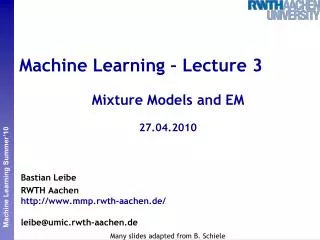
Machine Learning – Lecture 3 Mixture Models and EM 27.04.2010 Bastian Leibe RWTH Aachen http://www.mmp.rwth-aachen.de/ leibe@umic.rwth-aachen.de Many slides adapted from B. Schiele TexPoint fonts used in EMF. Read the TexPoint manual before you delete this box.: AAAAAAAAAAAAAAAAAAAAAAAAAAA
Announcements • Exercise 1 due tonight • Bayes decision theory • Maximum Likelihood • Kernel density estimation / k-NN Submit your results to Georgios until this evening. • Exercise modalities • Need to reach 50% of the points to qualify for the exam! • You can work in teams of up to 2 people. • If you work in a team • Turn in a single solution • But put both names on it B. Leibe
Course Outline • Fundamentals (2 weeks) • Bayes Decision Theory • Probability Density Estimation • Discriminative Approaches (4 weeks) • Linear Discriminant Functions • Support Vector Machines • Ensemble Methods & Boosting • Randomized Trees, Forests & Ferns • Generative Models (4 weeks) • Bayesian Networks • Markov Random Fields • Unifying Perspective (2 weeks) B. Leibe
Recap: Gaussian (or Normal) Distribution • One-dimensional case • Mean ¹ • Variance ¾2 • Multi-dimensional case • Mean ¹ • Covariance § B. Leibe Image source: C.M. Bishop, 2006
Recap: Maximum Likelihood Approach • Computation of the likelihood • Single data point: • Assumption: all data points are independent • Log-likelihood • Estimation of the parameters µ (Learning) • Maximize the likelihood (=minimize the negative log-likelihood) Take the derivative and set it to zero. B. Leibe Slide credit: Bernt Schiele
Recap: Bayesian Learning Approach • Bayesian view: • Consider the parameter vector µ as a random variable. • When estimating the parameters, what we compute is Assumption: given µ, thisdoesn’t depend on X anymore This is entirely determined by the parameter µ (i.e. by the parametric form of the pdf). B. Leibe Slide adapted from Bernt Schiele
Recap: Bayesian Learning Approach • Discussion • The more uncertain we are about µ, the more we average over all possible parameter values. Likelihood of the parametric form µ given the data set X. Estimate for x based onparametric form µ Prior for the parameters µ Normalization: integrate over all possible values of µ B. Leibe
Recap: Histograms • Basic idea: • Partition the data space into distinct bins with widths ¢i and count the number of observations, ni, in each bin. • Often, the same width is used for all bins, ¢i = ¢. • This can be done, in principle, for any dimensionality D… …but the requirednumber of binsgrows exponen-tially with D! B. Leibe Image source: C.M. Bishop, 2006
Recap: Kernel Methods • Kernel methods • Place a kernel windowkat location x and count how many data points fall inside it. fixed V determine K fixed K determine V Kernel Methods K-Nearest Neighbor • K-Nearest Neighbor • Increase the volume Vuntil the K next datapoints are found. B. Leibe Slide adapted from Bernt Schiele
Topics of This Lecture • Mixture distributions • Mixture of Gaussians (MoG) • Maximum Likelihood estimation attempt • K-Means Clustering • Algorithm • Applications • EM Algorithm • Credit assignment problem • MoG estimation • EM Algorithm • Interpretation of K-Means • Technical advice • Applications B. Leibe
Mixture Distributions • A single parametric distribution is often not sufficient • E.g. for multimodal data Single Gaussian Mixture of two Gaussians B. Leibe Image source: C.M. Bishop, 2006
Mixture of Gaussians (MoG) • Sum of M individual Normal distributions • In the limit, every smooth distribution can be approximated this way (if M is large enough) B. Leibe Slide credit: Bernt Schiele
Mixture of Gaussians with and . • Notes • The mixture density integrates to 1: • The mixture parameters are Likelihood of measurement xgiven mixture component j Prior ofcomponent j B. Leibe Slide adapted from Bernt Schiele
Mixture of Gaussians (MoG) • “Generative model” “Weight” of mixturecomponent 1 3 2 Mixturecomponent Mixture density B. Leibe Slide credit: Bernt Schiele
Mixture of Multivariate Gaussians B. Leibe Image source: C.M. Bishop, 2006
Mixture of Multivariate Gaussians • Multivariate Gaussians • Mixture weights / mixture coefficients: with and • Parameters: B. Leibe Slide credit: Bernt Schiele Image source: C.M. Bishop, 2006
Mixture of Multivariate Gaussians • “Generative model” 3 1 2 B. Leibe Slide credit: Bernt Schiele Image source: C.M. Bishop, 2006
Mixture of Gaussians – 1st Estimation Attempt • Maximum Likelihood • Minimize • Let’s first look at ¹j: • We can already see that this will be difficult, since This will cause problems! B. Leibe Slide adapted from Bernt Schiele
Mixture of Gaussians – 1st Estimation Attempt • Minimization: • We thus obtain “responsibility” ofcomponent j for xn B. Leibe
Mixture of Gaussians – 1st Estimation Attempt • But… • I.e. there is no direct analytical solution! • Complex gradient function (non-linear mutual dependencies) • Optimization of one Gaussian depends on all other Gaussians! • It is possible to apply iterative numerical optimization here, but in the following, we will see a simpler method. B. Leibe
Mixture of Gaussians – Other Strategy • Other strategy: • Observed data: • Unobserved data: 1 111 22 2 2 • Unobserved = “hidden variable”: j|x • 1 111 00 0 0 • 0 000 11 1 1 B. Leibe Slide credit: Bernt Schiele
Mixture of Gaussians – Other Strategy • Assuming we knew the values of the hidden variable… ML for Gaussian #1 ML for Gaussian #2 assumed known 1 111 22 2 2 j • 1 111 00 0 0 • 0 000 11 1 1 B. Leibe Slide credit: Bernt Schiele
Mixture of Gaussians – Other Strategy • Assuming we knew the mixture components… • Bayes decision rule: Decide j = 1 if assumed known 1 111 22 2 2 j B. Leibe Slide credit: Bernt Schiele
Mixture of Gaussians – Other Strategy • Chicken and egg problem – what comes first? • In order to break the loop, we need an estimate for j. • E.g. by clustering… We don’t know any of those! 1 111 22 2 2 j B. Leibe Slide credit: Bernt Schiele
Clustering with Hard Assignments • Let’s first look at clustering with “hard assignments” B. Leibe Slide credit: Bernt Schiele
Topics of This Lecture • Mixture distributions • Mixture of Gaussians (MoG) • Maximum Likelihood estimation attempt • K-Means Clustering • Algorithm • Applications • EM Algorithm • Credit assignment problem • MoG estimation • EM Algorithm • Interpretation of K-Means • Technical advice • Applications B. Leibe
K-Means Clustering • Iterative procedure • Initialization: pick K arbitrarycentroids (cluster means) • Assign each sample to the closestcentroid. • Adjust the centroids to be themeans of the samples assignedto them. • Go to step 2 (until no change) • Algorithm is guaranteed toconverge after finite #iterations. • Local optimum • Final result depends on initialization. B. Leibe Slide credit: Bernt Schiele
K-Means – Example with K=2 B. Leibe Image source: C.M. Bishop, 2006
K-Means Clustering • K-Means optimizes the followingobjective function: • where • In practice, this procedure usually converges quickly to a local optimum. B. Leibe Image source: C.M. Bishop, 2006
Example Application: Image Compression Take each pixelas one data point. K-MeansClustering Set the pixel colorto the cluster mean. B. Leibe Image source: C.M. Bishop, 2006
Example Application: Image Compression K = 2 K = 3 K =10 Original image B. Leibe Image source: C.M. Bishop, 2006
Summary K-Means • Pros • Simple, fast to compute • Converges to local minimum of within-cluster squared error • Problem cases • Setting k? • Sensitive to initial centers • Sensitive to outliers • Detects spherical clusters only • Extensions • Speed-ups possible through efficient search structures • General distance measures: k-medioids B. Leibe Slide credit: Kristen Grauman
Topics of This Lecture • Mixture distributions • Mixture of Gaussians (MoG) • Maximum Likelihood estimation attempt • K-Means Clustering • Algorithm • Applications • EM Algorithm • Credit assignment problem • MoG estimation • EM Algorithm • Interpretation of K-Means • Technical advice • Applications B. Leibe
EM Clustering • Clustering with “soft assignments” • Expectation step of the EM algorithm 0.99 0.8 0.2 0.01 0.01 0.2 0.8 0.99 B. Leibe Slide credit: Bernt Schiele
EM Clustering • Clustering with “soft assignments” • Maximization step of the EM algorithm 0.99 0.8 0.2 0.01 Maximum Likelihoodestimate 0.01 0.2 0.8 0.99 B. Leibe Slide credit: Bernt Schiele
Credit Assignment Problem • “Credit Assignment Problem” • If we are just given x, we don’t know which mixture component this example came from • We can however evaluate the posterior probability that an observed x was generated from the first mixture component. B. Leibe Slide credit: Bernt Schiele
Mixture Density Estimation Example • Example • Assume we want to estimate a 2-component MoG model • If each sample in the training setwere labeled j2{1,2} according towhich mixture component (1 or 2)had generated it, then theestimation would be easy. • Labeled examples= no credit assignment problem. B. Leibe Slide credit: Bernt Schiele
Mixture Density Estimation Example • When examples are labeled, we can estimate the Gaussians independently • Using Maximum Likelihood estimation for single Gaussians. • Notation • Let li be the label for sample xi • Let N be the number of samples • Let Nj be the number of samples labeled j • Then for each j2{1,2} we set B. Leibe Slide credit: Bernt Schiele
Mixture Density Estimation Example • Of course, we don’t have such labels li… • But we can guess what the labels might be based on our current mixture distribution estimate (credit assignment problem). • We get softlabels or posterior probabilities of which Gaussian generated which example: • When the Gaussians are almostidentical (as in the figure), then for almost any given sample xi. Even small differences can help todetermine how to update the Gaussians. B. Leibe Slide credit: Bernt Schiele
EM Algorithm • Expectation-Maximization (EM) Algorithm • E-Step: softly assign samples to mixture components • M-Step: re-estimate the parameters (separately for each mixture component) based on the soft assignments = soft number of samples labeled j B. Leibe Slide adapted from Bernt Schiele
EM Algorithm – An Example B. Leibe Image source: C.M. Bishop, 2006
EM – Technical Advice • When implementing EM, we need to take care to avoid singularities in the estimation! • Mixture components may collapse on single data points. • E.g. consider the case (this also holds in general) • Assume component j is exactly centered on data point xn. This data point will then contribute a term in the likelihood function • For ¾j! 0, this term goes to infinity! Need to introduce regularization • Enforce minimum width for the Gaussians B. Leibe Image source: C.M. Bishop, 2006
EM – Technical Advice (2) • EM is very sensitive to the initialization • Will converge to a local optimum of E. • Convergence is relatively slow. Initialize with k-Means to get better results! • k-Means is itself initialized randomly, will also only find a local optimum. • But convergence is much faster. • Typical procedure • Run k-Means M times (e.g. M = 10-100). • Pick the best result (lowest error J). • Use this result to initialize EM • Set ¹j to the corresponding cluster mean from k-Means. • Initialize §j to the sample covariance of the associated data points. B. Leibe
K-Means Clustering Revisited • Interpreting the procedure • Initialization: pick K arbitrarycentroids (cluster means) • Assign each sample to the closestcentroid. • Adjust the centroids to be themeans of the samples assignedto them. • Go to step 2 (until no change) (E-Step) (M-Step) B. Leibe
K-Means Clustering Revisited • K-Means clustering essentially corresponds to a Gaussian Mixture Model (MoG or GMM) estimation with EM whenever • The covariances are of the K Gaussians are set to §j=¾2I • For some small, fixed ¾2 k-Means MoG B. Leibe Slide credit: Bernt Schiele
Summary: Gaussian Mixture Models • Properties • Very general, can represent any (continuous) distribution. • Once trained, very fast to evaluate. • Can be updated online. • Problems / Caveats • Some numerical issues in the implementation Need to apply regularization in order to avoid singularities. • EM for MoG is computationally expensive • Especially for high-dimensional problems! • More computational overhead and slower convergence than k-Means • Results very sensitive to initialization Run k-Means for some iterations as initialization! • Need to select the number of mixture components K. Model selection problem (see Lecture 10) B. Leibe
Topics of This Lecture • Mixture distributions • Mixture of Gaussians (MoG) • Maximum Likelihood estimation attempt • K-Means Clustering • Algorithm • Applications • EM Algorithm • Credit assignment problem • MoG estimation • EM Algorithm • Interpretation of K-Means • Technical advice • Applications B. Leibe
Applications • Mixture models are used in many practical applications. • Wherever distributions with complexor unknown shapes need to berepresented… • Popular application in Computer Vision • Model distributions of pixel colors. • Each pixel is one data point in e.g. RGB space. Learn a MoG to represent the class-conditional densities. Use the learned models to classify other pixels. B. Leibe Image source: C.M. Bishop, 2006
Gaussian Mixture Application: Background Model for Tracking • Train background MoG for each pixel • Model “common“ appearance variation for each background pixel. • Initialization with an empty scene. • Update the mixtures over time • Adapt to lighting changes, etc. • Used in many vision-based trackingapplications • Anything that cannot be explainedby the background model is labeledas foreground (=object). • Easy segmentation if camera is fixed. C. Stauffer, E. Grimson, Learning Patterns of Activity Using Real-Time Tracking, IEEE Trans. PAMI, 22(8):747-757, 2000. B. Leibe Image Source: Daniel Roth, Tobias Jäggli
Application: Image Segmentation • User assisted image segmentation • User marks two regions for foreground and background. • Learn a MoG model for the color values in each region. • Use those models to classify all other pixels. Simple segmentation procedure(building block for more complex applications) B. Leibe